
E. Kh. Akhmedov, S. Razzaque, A. Yu. Smirnov · JHEP 02 (2013) 082
Mass hierarchy, 2-3 mixing and CP-phase with Huge Atmospheric Neutrino Detectors
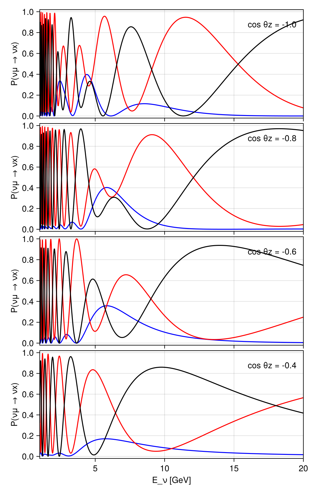
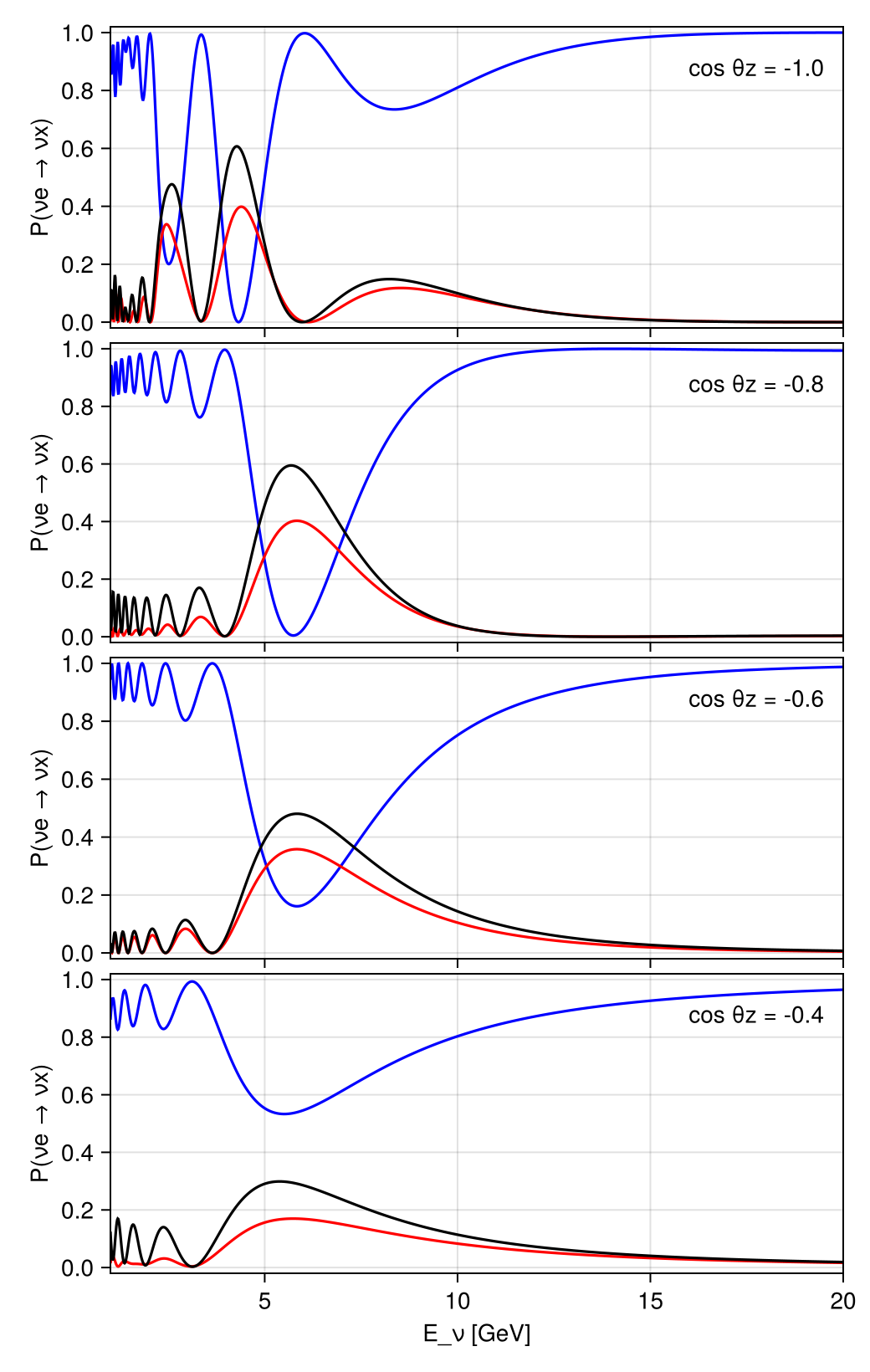
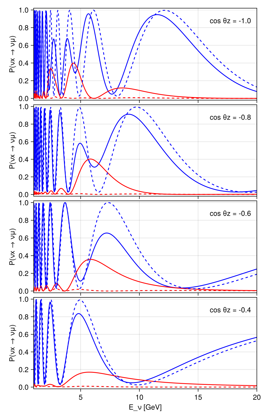
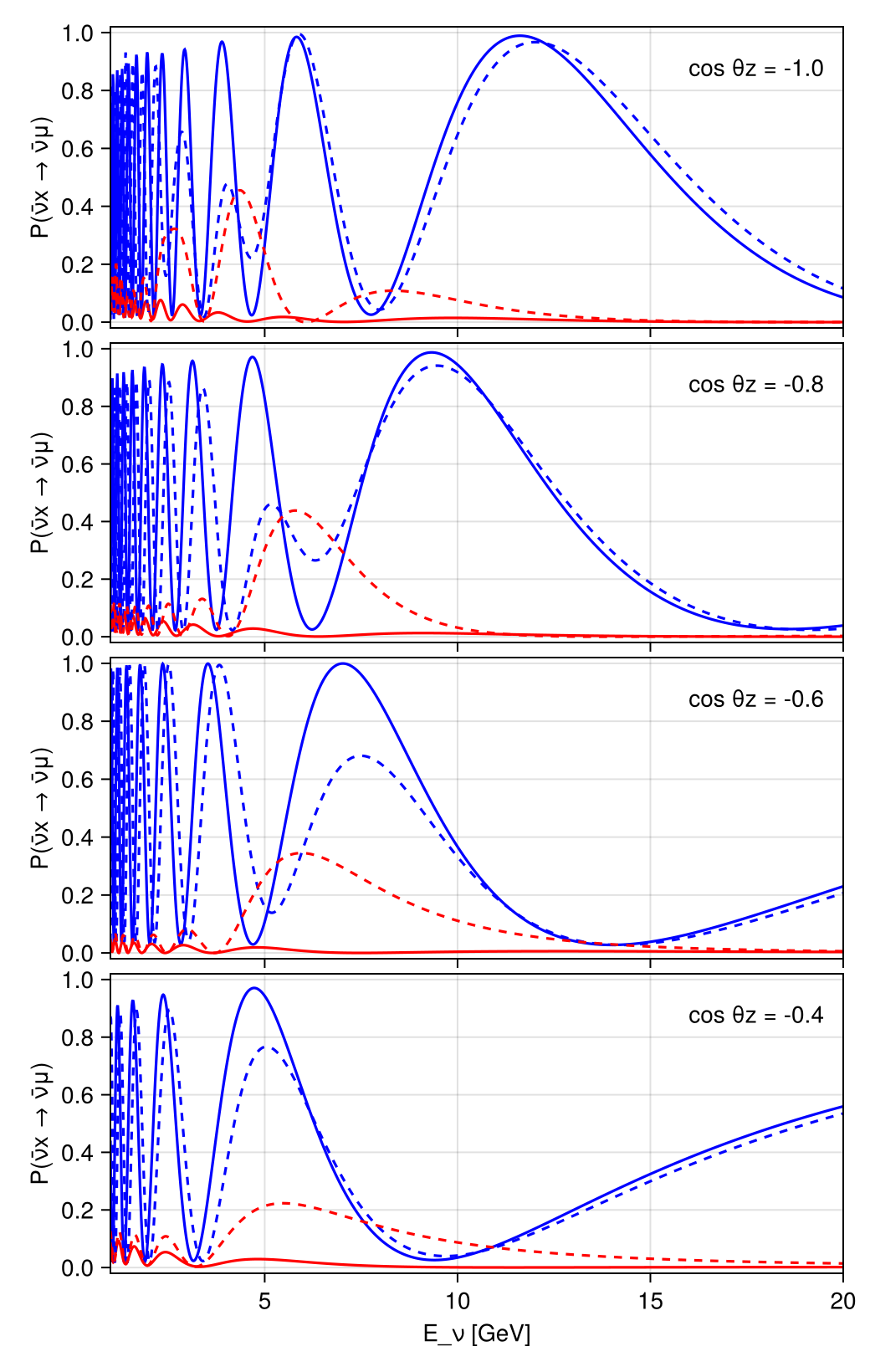
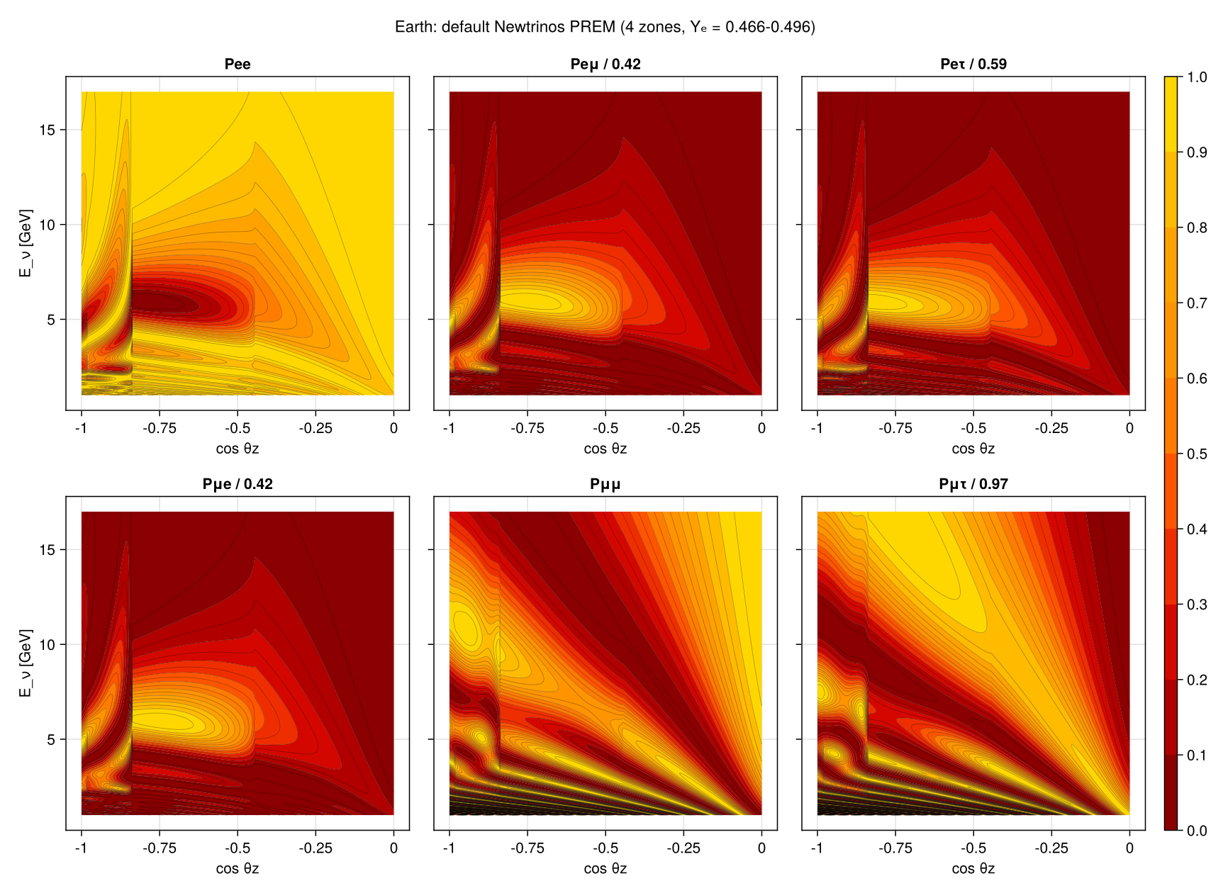
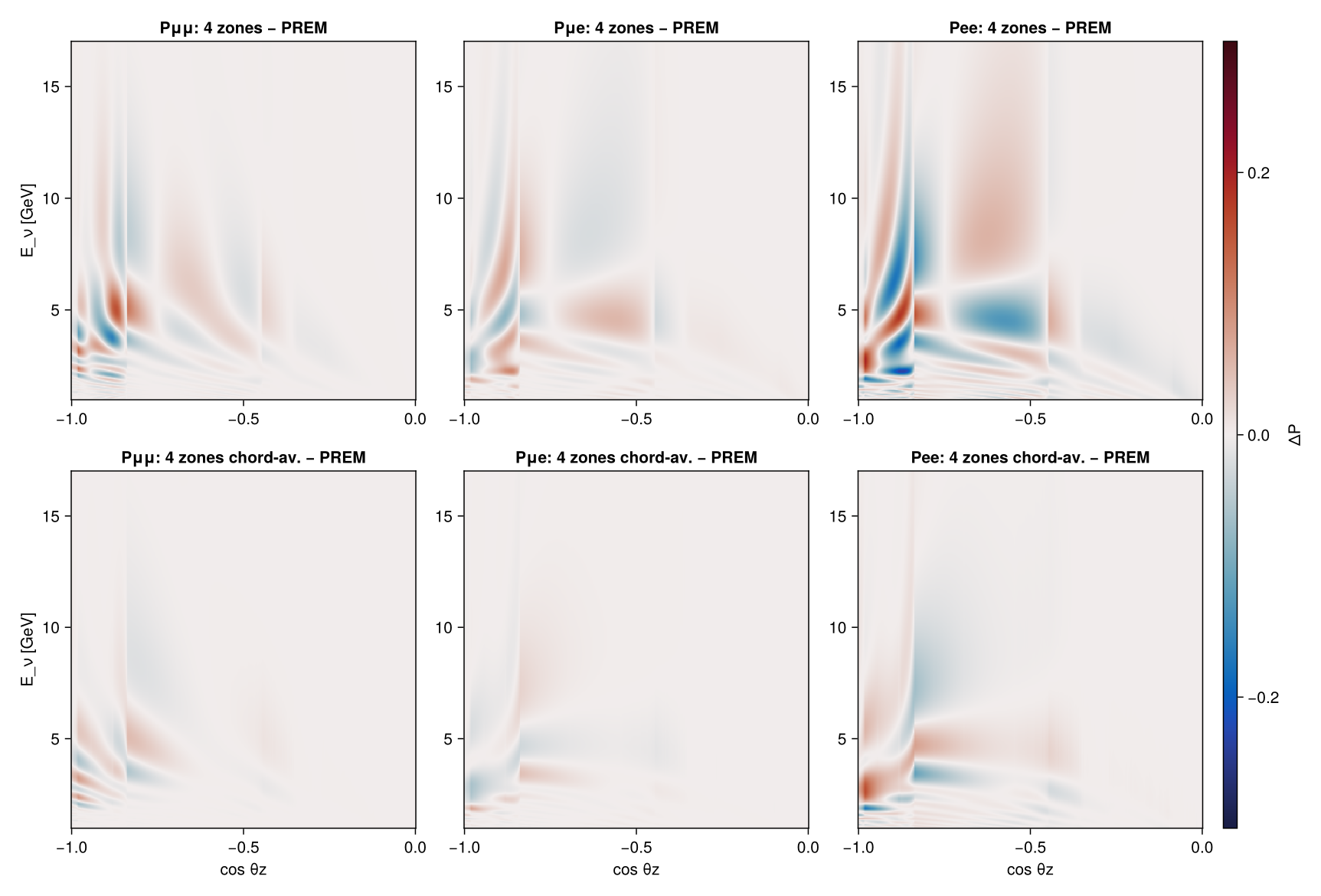
Three-flavour oscillation probabilities of atmospheric neutrinos crossing the Earth (modules osc with standard matter interactions and earth_layers): probabilities vs. energy at fixed zenith angles for both mass orderings, and the E–cos θ_z oscillograms with the MSW resonance in the mantle and the parametric enhancement for core-crossing trajectories. A second set of figures shows how much the default four-zone Newtrinos Earth changes the probabilities compared with the full PREM profile (PREM zoned at its density discontinuities with chord-averaged densities), with and without chord averaging of the four zones.
Figures
νμ → νe, νμ, ντ vs. energy, normal ordering · Fig. 1 (left)
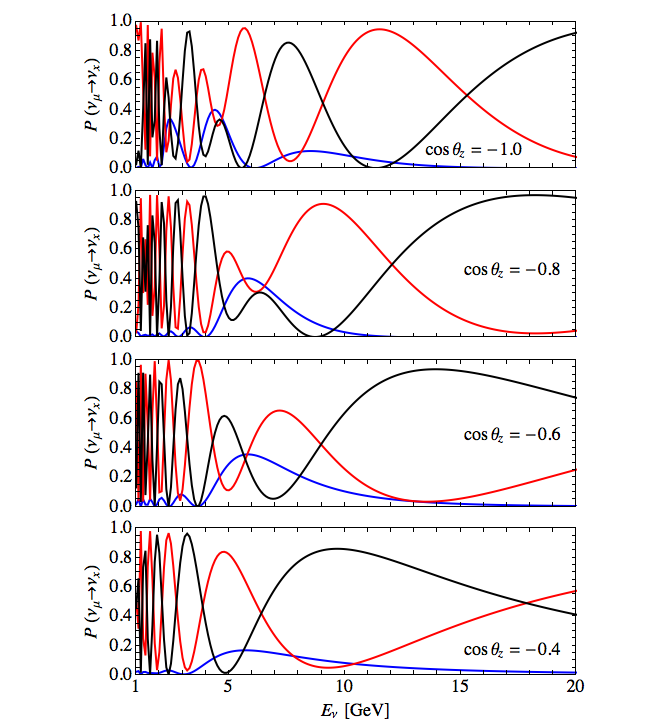
Original figure: E. Kh. Akhmedov, S. Razzaque, A. Yu. Smirnov, JHEP 02 (2013) 082, Fig. 1 (left), doi:10.1007/JHEP02(2013)082. Not our work; shown for comparison, all rights with the authors and publisher.
νe → νe, νμ, ντ vs. energy, normal ordering · Fig. 1 (right)
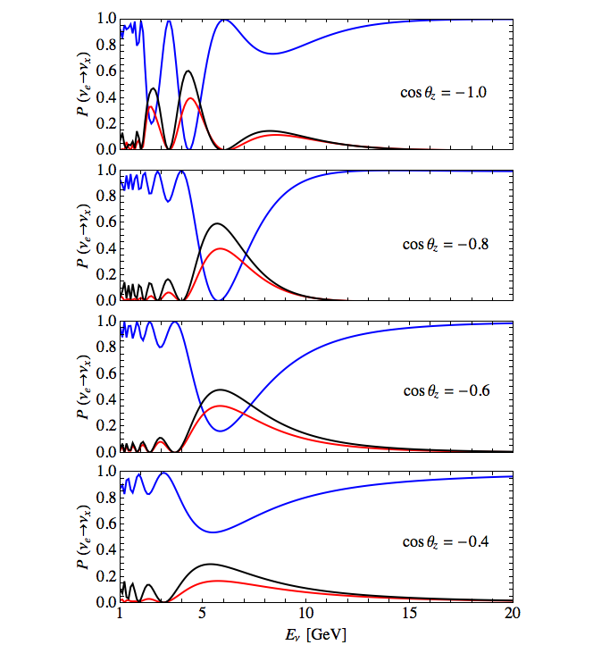
Original figure: E. Kh. Akhmedov, S. Razzaque, A. Yu. Smirnov, JHEP 02 (2013) 082, Fig. 1 (right), doi:10.1007/JHEP02(2013)082. Not our work; shown for comparison, all rights with the authors and publisher.
νμ → νμ (blue) and νe → νμ (red), NO solid, IO dashed · Fig. 2 (left)
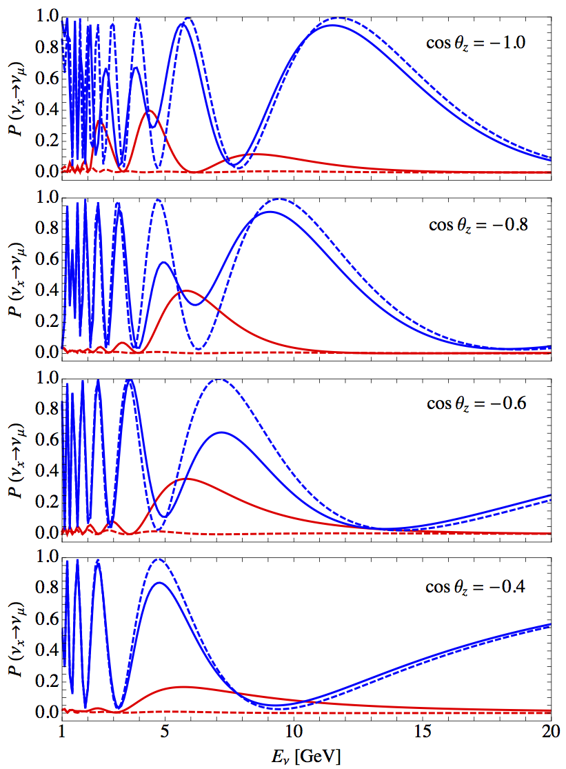
Original figure: E. Kh. Akhmedov, S. Razzaque, A. Yu. Smirnov, JHEP 02 (2013) 082, Fig. 2 (left), doi:10.1007/JHEP02(2013)082. Not our work; shown for comparison, all rights with the authors and publisher.
Antineutrinos: ν̄μ → ν̄μ and ν̄e → ν̄μ, NO solid, IO dashed · Fig. 2 (right)
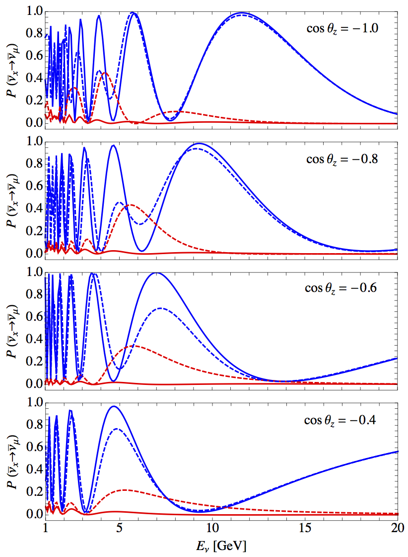
Original figure: E. Kh. Akhmedov, S. Razzaque, A. Yu. Smirnov, JHEP 02 (2013) 082, Fig. 2 (right), doi:10.1007/JHEP02(2013)082. Not our work; shown for comparison, all rights with the authors and publisher.
Oscillograms of the Earth, normal ordering · Fig. 3
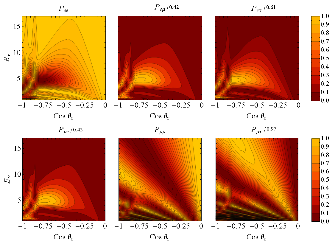
Original figure: E. Kh. Akhmedov, S. Razzaque, A. Yu. Smirnov, JHEP 02 (2013) 082, Fig. 3, doi:10.1007/JHEP02(2013)082. Not our work; shown for comparison, all rights with the authors and publisher.
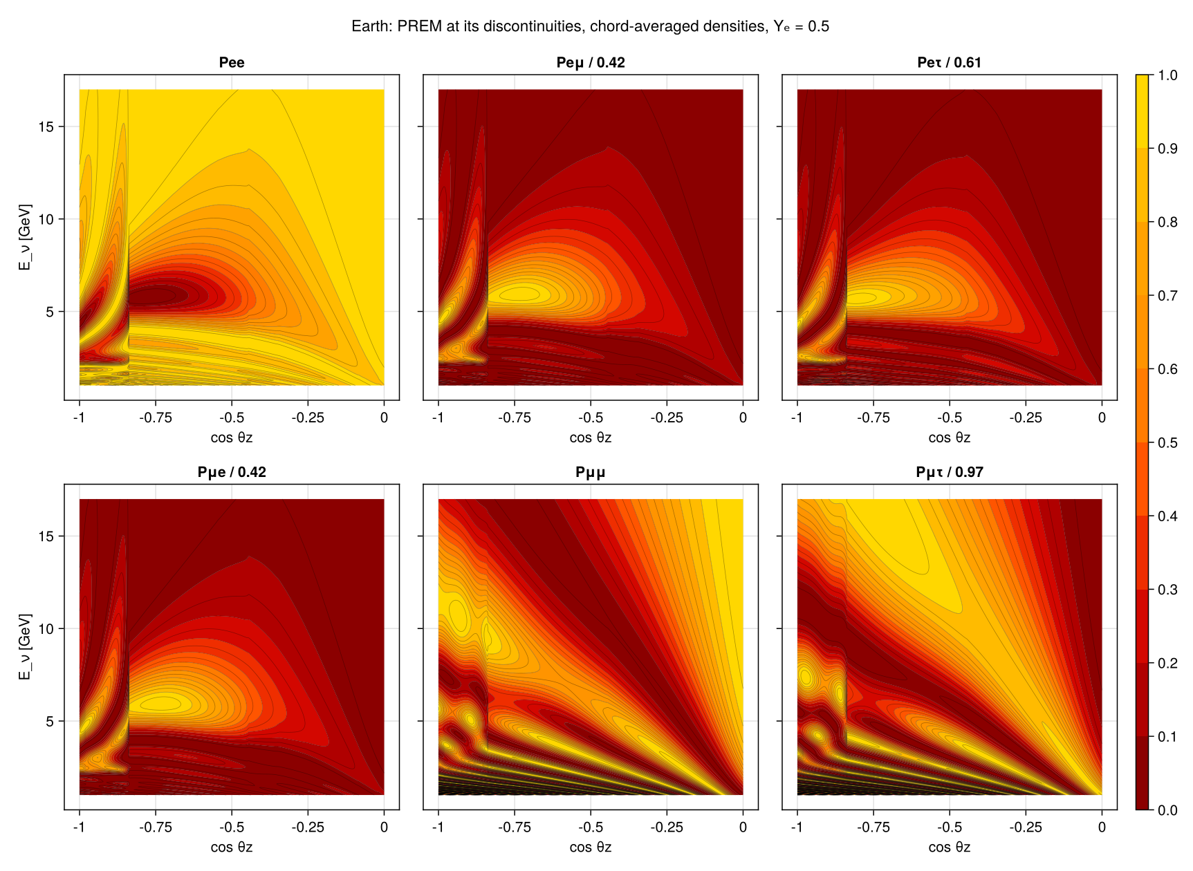
The same oscillograms with the default four-zone Newtrinos Earth · not in the paper
not in the paper
Probability difference to the full PREM profile (same Yₑ): four zones (top) and four chord-averaged zones (bottom) · not in the paper
not in the paper
Known limitations
- Reproduction conventions inferred from the paper's own curves: the quoted 2.35·10⁻³ eV² is used as Δm²₃₁ (the paper's formulae use Δ = Δm²₃₁/2E), and Yₑ = 0.5 throughout the Earth. With Δm²₃₁ = Δm²₃₂ + Δm²₂₁ the extrema shift up by ~3 % in energy, and with Yₑ = 0.466 in the core the core-crossing amplitudes change visibly (e.g. the second Pμe maximum at cos θ_z = −1 falls from 0.12 to 0.08).
- The paper-like Earth is the native Newtrinos PREM_discontinuities zoning with chord-averaged densities (compute_chord_paths, pieces ≤ 100 km), which follows the continuous PREM profile; Yₑ = 0.5 for the paper's figures. Analyses use the default Newtrinos Earth, four zone-averaged constant-density zones. Compared with the full profile (same Yₑ), that shifts the probabilities by up to |ΔP| ≈ 0.24 (Pee) for core-crossing and near-core trajectories, with visible steps at the zone boundaries (cos θ_z ≈ −0.45 and −0.84); mean |ΔP| over the plane 0.007–0.018. Chord-averaging the four zones reduces this to max 0.07–0.17 and mean 0.003–0.007. See the last two figures.
- In the paper's Fig. 3 the mantle resonance (the minimum of Pee) appears near 4.8 GeV. The paper's own Figs. 1 and 2, and our calculation, put it near 5.8 GeV at cos θ_z = −0.8. The channel maxima quoted in Fig. 3 (Peμ 0.42, Peτ 0.61, Pμτ 0.97) are reproduced (0.424, 0.607, 0.972).
Reproduce
git clone https://github.com/Newtrinos-org/Newtrinos.jl.git && cd Newtrinos.jl && git checkout e1b5a89439- Download reproduce.jl into an empty directory.
julia -t 8 --project=/path/to/Newtrinos.jl reproduce.jl
# Atmospheric neutrino oscillograms of the Earth with Newtrinos.jl (modules `osc` with standard matter
# interactions and `earth_layers`), compared with Akhmedov, Razzaque, Smirnov, JHEP 02 (2013) 082, Figs. 1-3.
# Run from this directory with the Newtrinos.jl environment at the pinned commit:
#   julia --project=<path to Newtrinos.jl> reproduce.jl
using Newtrinos, CairoMakie, CSV, DataFrames, StructArrays, Printf

cd(@__DIR__); mkpath("ours"); mkpath("results")

# oscillation parameters of the paper (Sec. 2): "Δm²₃₂" = 2.35e-3 eV², Δm²₂₁ = 7.6e-5 eV², sin²θ₂₃ = 0.42,
# sin²θ₁₂ = 0.312, sin²θ₁₃ = 0.025, δ = 0. The positions of the extrema in the paper's Fig. 2 are reproduced
# when 2.35e-3 eV² is used as Δm²₃₁ (the paper's formulae use Δ = Δm²₃₁ / 2E); IH: Δm²₃₁ → -Δm²₃₁.
const Δm² = 2.35e-3
base = (θ₁₂ = asin(sqrt(0.312)), θ₁₃ = asin(sqrt(0.025)), θ₂₃ = asin(sqrt(0.42)), δCP = 0.0, Δm²₂₁ = 7.6e-5)
params = (NH = (; base..., Δm²₃₁ = Δm²), IH = (; base..., Δm²₃₁ = -Δm²))

osc = Newtrinos.osc.configure(Newtrinos.osc.OscillationConfig(interaction = Newtrinos.osc.SI()))
earth = Newtrinos.earth_layers.configure()

# (a) the default Newtrinos Earth: PREM averaged into four constant-density zones (as used in the analyses)
layers_default = earth.compute_layers()

# (b) close to the paper's full PREM profile: PREM zoned at its density discontinuities, with the density of
#     every chord segment averaged along the chord (pieces ≤ 100 km), electron fraction ye_core / ye_mantle
function chord_earth(ye_core, ye_mantle)
    z = Newtrinos.earth_layers.PREM_discontinuities().zones
    cfg = Newtrinos.earth_layers.PREM(zones = z, p_fractions = [z[i] >= 5.6 ? ye_core : ye_mantle for i in 1:length(z)-1])
    e = Newtrinos.earth_layers.configure(cfg)
    (earth = e, layers = e.compute_layers(), max_length = 100.0)
end
layers_paper = chord_earth(0.5, 0.5)        # the paper's amplitudes at cos θz = -1 require Yₑ = 0.5 in the core
layers_fine = chord_earth(0.466, 0.494)     # same Yₑ as the default Newtrinos zones: isolates the layering
# (c) the default four zones, but with chord-averaged densities
layers_chord = (earth = earth, layers = layers_default, max_length = Inf)

const FL = ("e", "μ", "τ")
prob(E, cz, layers, par; anti = false) = osc.osc_prob(E, earth.compute_paths(cz, layers), layers, par; anti)
prob(E, cz, m::NamedTuple, par; anti = false) =
    osc.osc_prob(E, m.earth.compute_chord_paths(cz, m.layers; max_length = m.max_length)..., par; anti)

# ---------------- Figs. 1 and 2: P vs E at four zenith angles ----------------
E1 = collect(range(1, 20, length = 1500))
CZ1 = [-1.0, -0.8, -0.6, -0.4]
P = Dict((h, a) => prob(E1, CZ1, layers_paper, params[h]; anti = a) for h in (:NH, :IH), a in (false, true))

function panel_column(fname, ylabel, curves)
    fig = Figure(size = (520, 820))
    for (j, cz) in enumerate(CZ1)
        ax = Axis(fig[j, 1], ylabel = ylabel, limits = (1, 20, -0.02, 1.02), yticks = 0:0.2:1,
                  xlabel = j == 4 ? "E_ν [GeV]" : "", xticklabelsvisible = j == 4)
        for c in curves
            lines!(ax, E1, c.p[:, j]; color = c.color, linestyle = c.style, linewidth = 1.6)
        end
        text!(ax, 19.5, 0.88, text = @sprintf("cos θz = %.1f", cz), align = (:right, :center), fontsize = 14)
    end
    rowgap!(fig.layout, 4)
    save(fname, fig, px_per_unit = 2)
end
col = (e = :blue, μ = :red, τ = :black)
Pd = P[(:NH, false)]
panel_column("ours/fig1a_numu.png", "P(νμ → νx)", [(p = Pd[:, :, 2, i], color = col[i], style = :solid) for i in 1:3])
panel_column("ours/fig1b_nue.png", "P(νe → νx)", [(p = Pd[:, :, 1, i], color = col[i], style = :solid) for i in 1:3])
for (a, tag, lab) in ((false, "fig2a_nu", "P(νx → νμ)"), (true, "fig2b_nubar", "P(ν̄x → ν̄μ)"))
    curves = [(p = P[(h, a)][:, :, α, 2], color = c, style = s)
              for (h, s) in ((:NH, :solid), (:IH, :dash)) for (α, c) in ((2, :blue), (1, :red))]
    panel_column("ours/$tag.png", lab, curves)
end

# ---------------- Fig. 3: oscillograms (NH, neutrinos), normalised to the maximum in the panel ----------------
E3 = collect(range(1, 17, length = 400))
CZ3 = collect(range(-1, 0, length = 400))
P3paper = prob(E3, CZ3, layers_paper, params.NH)
P3 = prob(E3, CZ3, layers_default, params.NH)
P3fine = prob(E3, CZ3, layers_fine, params.NH)
P3chord = prob(E3, CZ3, layers_chord, params.NH)
channels = [(1, 1), (1, 2), (1, 3), (2, 1), (2, 2), (2, 3)]
cmap = cgrad([:darkred, :red3, :orangered, :darkorange, :orange, :gold], 10, categorical = true)
function oscillograms(fname, P3, label)
    fig = Figure(size = (1150, 840))
    for (k, (α, β)) in enumerate(channels)
        z = P3[:, :, α, β]'
        zmax = α == β ? 1.0 : maximum(z)
        ttl = α == β ? "P$(FL[α])$(FL[β])" : @sprintf("P%s%s / %.2f", FL[α], FL[β], zmax)
        ax = Axis(fig[(k - 1) ÷ 3 + 1, (k - 1) % 3 + 1], title = ttl, xlabel = "cos θz",
                  ylabel = k in (1, 4) ? "E_ν [GeV]" : "", yticklabelsvisible = k in (1, 4),
                  xticks = ([-1, -0.75, -0.5, -0.25, 0], ["-1", "-0.75", "-0.5", "-0.25", "0"]))
        contourf!(ax, CZ3, E3, z ./ zmax, levels = 0:0.1:1, colormap = cmap)
        contour!(ax, CZ3, E3, z ./ zmax, levels = 0.05:0.05:0.95, color = (:black, 0.35), linewidth = 0.5)
    end
    Colorbar(fig[1:2, 4], colormap = cmap, limits = (0, 1), ticks = 0:0.1:1)
    Label(fig[0, 1:3], label, fontsize = 15)
    save(fname, fig, px_per_unit = 1.5)
end
oscillograms("ours/fig3_oscillograms.png", P3paper, "Earth: PREM at its discontinuities, chord-averaged densities, Yₑ = 0.5")
oscillograms("ours/fig3_oscillograms_4zone.png", P3, "Earth: default Newtrinos PREM (4 zones, Yₑ = 0.466-0.496)")

# maxima quoted in the paper's Fig. 3 titles: Peμ 0.42, Peτ 0.61, Pμe 0.42, Pμτ 0.97
paper_max = Dict((1, 2) => 0.42, (1, 3) => 0.61, (2, 1) => 0.42, (2, 3) => 0.97)
rows = map(collect(paper_max)) do ((α, β), pm)
    (channel = "P$(FL[α])$(FL[β])", paper_max = pm,
     newtrinos_max = round(maximum(P3paper[:, :, α, β]), digits = 3),
     newtrinos_max_default_earth = round(maximum(P3[:, :, α, β]), digits = 3))
end
sort!(rows, by = r -> r.channel)
CSV.write("results/fig3_channel_maxima.csv", DataFrame(rows))

# impact of the Earth layering: |P(model) - P(reference PREM)| over the Fig. 3 plane, same Yₑ
lay = [(channel = "P$(FL[α])$(FL[β])", model = m,
        max_abs_diff = round(maximum(abs.(Pm[:, :, α, β] .- P3fine[:, :, α, β])), digits = 3),
        mean_abs_diff = round(sum(abs.(Pm[:, :, α, β] .- P3fine[:, :, α, β])) / length(Pm[:, :, α, β]), digits = 4))
       for (m, Pm) in (("4 zones", P3), ("4 zones chord-averaged", P3chord)) for (α, β) in channels]
CSV.write("results/layering_4zone_vs_fine.csv", DataFrame(lay))

fig = Figure(size = (1150, 780))
for (r, (Pm, lab)) in enumerate(((P3, "4 zones"), (P3chord, "4 zones chord-av.")))
    for (k, (α, β)) in enumerate(((2, 2), (2, 1), (1, 1)))
        local ax = Axis(fig[r, k], title = "P$(FL[α])$(FL[β]): $lab − PREM", xlabel = r == 2 ? "cos θz" : "",
                        ylabel = k == 1 ? "E_ν [GeV]" : "")
        hm = heatmap!(ax, CZ3, E3, (Pm[:, :, α, β] .- P3fine[:, :, α, β])', colormap = :balance, colorrange = (-0.3, 0.3))
        k == 3 && r == 1 && Colorbar(fig[1:2, 4], hm, label = "ΔP")
    end
end
save("ours/layering_difference.png", fig, px_per_unit = 1.5)

println("Fig. 3 channel maxima (paper vs Newtrinos paper-like Earth / default Earth):")
for r in rows
    @printf("  %s  %.2f  %.3f / %.3f\n", r.channel, r.paper_max, r.newtrinos_max, r.newtrinos_max_default_earth)
end
println("4-zone (and chord-averaged 4-zone) vs reference PREM Earth (same Yₑ), max |ΔP| over 1-17 GeV, cos θz ∈ [-1, 0]:")
for r in lay
    @printf("  %-24s %s  max %.3f  mean %.4f\n", r.model, r.channel, r.max_abs_diff, r.mean_abs_diff)
end
Provenance
| Newtrinos.jl commit | e1b5a89439 (osc (ThreeFlavour, SI), earth_layers) |
|---|---|
| Run date | 2026-10-11T10:28:07Z |
| Wall time | 4.2 min (8 threads) |
| Julia | 1.12.5 |
| Machine | AMD EPYC 7702P 64-Core Processor, 128 hardware threads, Linux |
| Environment | newtrinos_Manifest.toml · run.toml |
Downloads
CSV files hold one row per scan point: the scanned and profiled parameters
(sin2_theta23, dm2_32 in eV², dcp in rad, nuisance parameters), dchi2 = −2Δ log L
and the log-likelihood. JLD2 files contain the full NewtrinosResult objects.
| File | Size | SHA-256 |
|---|---|---|
| ours/fig1a_numu.png | 374.2 kB | 00e2d3b3591d… |
| ours/fig1b_nue.png | 236.5 kB | c9e9155833c0… |
| ours/fig2a_nu.png | 324.7 kB | faf25e39e526… |
| ours/fig2b_nubar.png | 329.8 kB | 18b7e952257a… |
| ours/fig3_oscillograms.png | 1.0 MB | fa1ea6d73a40… |
| ours/fig3_oscillograms_4zone.png | 1.0 MB | 777f67d43a95… |
| ours/layering_difference.png | 416.0 kB | aa49ece8ddb2… |
| results/fig3_channel_maxima.csv | 148 B | 8650a7c1c691… |
| results/layering_4zone_vs_fine.csv | 444 B | c79940915cfa… |