
P. B. Denton, H. Minakata, S. J. Parke · JHEP 06 (2016) 051
Compact Perturbative Expressions For Neutrino Oscillations in Matter
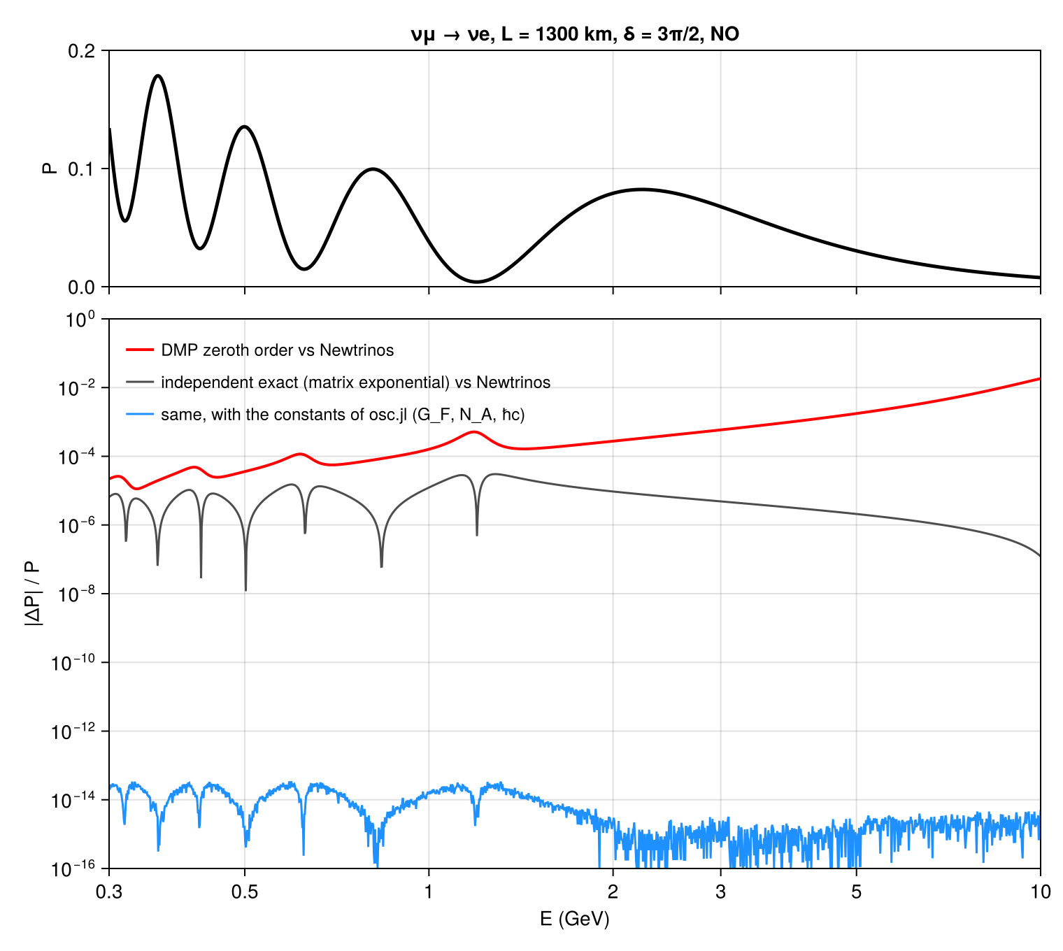
Three-flavour oscillation probabilities in constant-density matter from Newtrinos.jl (module osc, standard matter interactions, one constant-density layer) for the DUNE setting of the paper's Fig. 4 (L = 1300 km, Yₑρ = 1.4 g/cm³, δ = 3π/2, NO). They are compared with the zeroth-order Denton–Minakata–Parke expansion, implemented independently in reproduce.jl, and with an independent exact solution, the matrix exponential of the full Hamiltonian, for all nine channels of neutrinos and antineutrinos.
Figures
P(νμ → νe) for DUNE and the precision of the zeroth-order expansion · Fig. 4
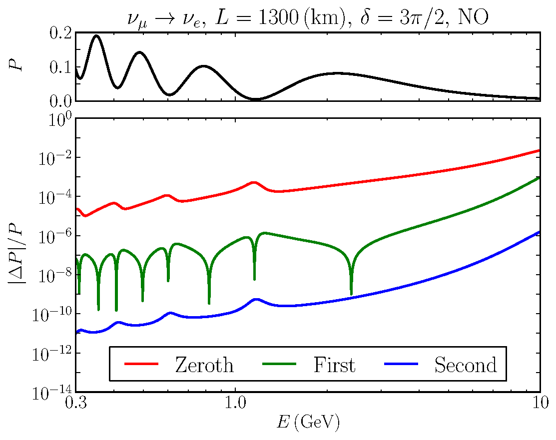
Original figure: P. B. Denton, H. Minakata, S. J. Parke, JHEP 06 (2016) 051, Fig. 4, doi:10.1007/JHEP06(2016)051. Not our work; shown for comparison, all rights with the authors and publisher.
Known limitations
- Newtrinos and the independent matrix exponential agree to 2·10⁻¹⁴ in all channels when both use the physical constants of osc.jl. With CODATA constants they differ by up to 1.4·10⁻⁶, almost entirely because osc.jl uses N_A = 6.022·10²³ mol⁻¹ (instead of 6.02214076·10²³), which scales the matter potential by −2.4·10⁻⁵.
- The fractional precision of the zeroth-order DMP expansion vs. Newtrinos follows the paper's red curve (≈ 2·10⁻⁵ at 0.3 GeV, a bump of ≈ 5·10⁻⁴ near 1.2 GeV, ≈ 2·10⁻² at 10 GeV); at the first oscillation maximum and minimum it is 3.4·10⁻⁴ and 5.0·10⁻⁴ (paper's Table 3: 5·10⁻⁴ and 4·10⁻⁴, with its own unlisted parameter values). The first- and second-order expansions are not implemented here.
- The paper does not list its oscillation parameters; typical 2016 values are used (sin²θ₁₂ = 0.31, sin²θ₁₃ = 0.022, sin²θ₂₃ = 0.5, Δm²₂₁ = 7.5·10⁻⁵ eV², Δm²₃₁ = 2.5·10⁻³ eV²). The matter potential is computed from G_F and N_A (1.5265·10⁻⁴ Yₑρ E eV²; the paper's eq. (2.3) quotes the rounded 1.52·10⁻⁴).
Reproduce
git clone https://github.com/Newtrinos-org/Newtrinos.jl.git && cd Newtrinos.jl && git checkout de27463fde- Download reproduce.jl into an empty directory.
julia -t 8 --project=/path/to/Newtrinos.jl reproduce.jl
# Three-flavour oscillation probabilities in constant-density matter with Newtrinos.jl (module `osc`, standard matter
# interactions) compared with the perturbative expansion of Denton, Minakata, Parke, JHEP 06 (2016) 051, Fig. 4, and
# with an independent exact solution (matrix exponential of the full Hamiltonian).
# Run from this directory with the Newtrinos.jl environment at the pinned commit:
#   julia --project=<path to Newtrinos.jl> reproduce.jl
using Newtrinos, CairoMakie, CSV, DataFrames, Printf, LinearAlgebra, StructArrays, ArraysOfArrays

cd(@__DIR__); mkpath("ours"); mkpath("results")

# DUNE setting of the paper's Fig. 4: L = 1300 km, Yₑρ = 1.4 g/cm³, δ = 3π/2, NO. The paper does not list its oscillation
# parameters; typical 2016 global-fit values are used.
const L, Yρ = 1300.0, 1.4
par = (θ₁₂ = asin(sqrt(0.31)), θ₁₃ = asin(sqrt(0.022)), θ₂₃ = asin(sqrt(0.5)), δCP = 3π / 2, Δm²₂₁ = 7.5e-5, Δm²₃₁ = 2.5e-3)
E = 10 .^ range(log10(0.3), 1, length = 1500)

# ---- Newtrinos: one constant-density layer (p_density = Yₑρ), one path of length L
osc = Newtrinos.osc.configure(Newtrinos.osc.OscillationConfig(interaction = Newtrinos.osc.SI()))
layers = StructArray{Newtrinos.Layer}(([7000.0], [Yρ], [Yρ]))
paths = VectorOfVectors{Newtrinos.Path}([StructArray{Newtrinos.Path}(([L], [1]))])
P_newtrinos(anti) = osc.osc_prob(E, paths, layers, par; anti)[:, 1, :, :]     # [E, α, β]

# ---- independent exact solution: S = exp(-i H L), H = [U diag(0, Δm²₂₁, Δm²₃₁) U† + diag(a, 0, 0)] / 2E
function pmns(p)
    s12, c12, s13, c13, s23, c23 = sin(p.θ₁₂), cos(p.θ₁₂), sin(p.θ₁₃), cos(p.θ₁₃), sin(p.θ₂₃), cos(p.θ₂₃)
    e = cis(p.δCP)
    [1 0 0; 0 c23 s23; 0 -s23 c23] * [c13 0 s13/e; 0 1 0; -s13*e 0 c13] * [c12 s12 0; -s12 c12 0; 0 0 1]
end
# a = 2√2 G_F N_e E [eV²] from G_F = 1.1663787e-5 GeV⁻², ħc = 1.97326980e-5 eV·cm, N_A = 6.02214076e23 mol⁻¹:
# 1.5265e-4 Yₑρ[g/cm³] E[GeV] (the paper's eq. (2.3) quotes the rounded 1.52e-4)
const GF_EVCM3 = 1.1663787e-23 * 1.97326980e-5^3
amatter(Egev; GF = GF_EVCM3, NA = 6.02214076e23) = 2 * sqrt(2) * GF * NA * Yρ * Egev * 1e9
const PHASE = 1 / (2 * 0.197326980)                         # Δm²[eV²] L[km] / E[GeV] → Δm²L/2E
# the same constants as osc.jl (G_F, N_A, 1/2ħc), to separate solver precision from the choice of constants
const NEWTRINOS_CONSTANTS = (GF = Newtrinos.osc.G_F, NA = Newtrinos.osc.N_A, phase = Newtrinos.osc.F_units)
function P_expm(Egev, anti; GF = GF_EVCM3, NA = 6.02214076e23, phase = PHASE)
    U = pmns(par); U = anti ? conj(U) : U
    a = (anti ? -1 : 1) * amatter(Egev; GF, NA)
    M = U * Diagonal([0, par.Δm²₂₁, par.Δm²₃₁]) * U' + Diagonal([a, 0, 0])     # 2E·H [eV²]
    S = exp(-im * M * L / Egev * phase)
    abs2.(transpose(S))                                       # P[α, β] = |S_βα|²
end

# ---- DMP zeroth order (Sec. 2): rotations U₂₃(θ₂₃, δ) U₁₃(φ) U₁₂(ψ), eigenvalues λ₁, λ₂, λ₃
function P_dmp0(Egev, anti)
    s12, c12, s13, c13 = sin(par.θ₁₂), cos(par.θ₁₂), sin(par.θ₁₃), cos(par.θ₁₃)
    δ = anti ? -par.δCP : par.δCP
    a = anti ? -amatter(Egev) : amatter(Egev)
    Δee = par.Δm²₃₁ - s12^2 * par.Δm²₂₁
    ε = par.Δm²₂₁ / Δee
    λa = a + (s13^2 + ε * s12^2) * Δee
    λb = ε * c12^2 * Δee
    λc = (c13^2 + ε * s12^2) * Δee
    sg = sign(Δee)
    λm = ((λa + λc) - sg * sqrt((λc - λa)^2 + 4 * (s13 * c13 * Δee)^2)) / 2
    λp = ((λa + λc) + sg * sqrt((λc - λa)^2 + 4 * (s13 * c13 * Δee)^2)) / 2
    λ0 = λb
    sφ, cφ = sqrt((λp - λc) / (λp - λm)), sqrt((λc - λm) / (λp - λm))
    φ = atan(sφ, cφ)
    cpt = cos(φ - par.θ₁₃)
    λ1 = ((λ0 + λm) - sqrt((λ0 - λm)^2 + 4 * (ε * cpt * c12 * s12 * Δee)^2)) / 2
    λ2 = ((λ0 + λm) + sqrt((λ0 - λm)^2 + 4 * (ε * cpt * c12 * s12 * Δee)^2)) / 2
    λ3 = λp
    sψ, cψ = sqrt((λ2 - λ0) / (λ2 - λ1)), sign(λ2 - λ1) * sqrt((λ0 - λ1) / (λ2 - λ1))
    ψ = atan(sψ, cψ)
    U = pmns((θ₁₂ = ψ, θ₁₃ = φ, θ₂₃ = par.θ₂₃, δCP = δ))
    phase = cis.(-[λ1, λ2, λ3] .* L ./ Egev .* PHASE)
    [abs2(sum(U[β, i] * conj(U[α, i]) * phase[i] for i in 1:3)) for α in 1:3, β in 1:3]
end

res = Dict()
for anti in (false, true)
    Pn = P_newtrinos(anti)
    Px = cat((P_expm(e, anti) for e in E)..., dims = 3)        # [α, β, E]
    Pd = cat((P_dmp0(e, anti) for e in E)..., dims = 3)
    Pa = cat((P_expm(e, anti; NEWTRINOS_CONSTANTS...) for e in E)..., dims = 3)
    res[anti] = (newtrinos = Pn, expm = permutedims(Px, (3, 1, 2)), dmp0 = permutedims(Pd, (3, 1, 2)),
                 expm_NA = permutedims(Pa, (3, 1, 2)))
end

# ---- Fig. 4: P(νμ → νe) and the fractional precision of the zeroth-order expansion
r = res[false]
Pme = r.newtrinos[:, 2, 1]
fig = Figure(size = (760, 680))
ET = ([0.3, 0.5, 1, 2, 3, 5, 10], ["0.3", "0.5", "1", "2", "3", "5", "10"])
ax1 = Axis(fig[1, 1], xscale = log10, xticks = ET, ylabel = "P", title = "νμ → νe, L = 1300 km, δ = 3π/2, NO", limits = (0.3, 10, 0, 0.2),
           xticklabelsvisible = false)
lines!(ax1, E, Pme, color = :black, linewidth = 2.5)
ax2 = Axis(fig[2, 1], xscale = log10, xticks = ET, yscale = log10, xlabel = "E (GeV)", ylabel = "|ΔP| / P", limits = (0.3, 10, 1e-16, 1),
           yticks = LogTicks(-16:2:0))
lines!(ax2, E, abs.(r.dmp0[:, 2, 1] .- Pme) ./ Pme, color = :red, linewidth = 2, label = "DMP zeroth order vs Newtrinos")
lines!(ax2, E, max.(abs.(r.expm[:, 2, 1] .- Pme) ./ Pme, 1e-16), color = :gray30, linewidth = 1.5,
       label = "independent exact (matrix exponential) vs Newtrinos")
lines!(ax2, E, max.(abs.(r.expm_NA[:, 2, 1] .- Pme) ./ Pme, 1e-16), color = :dodgerblue, linewidth = 1.5,
       label = "same, with the constants of osc.jl (G_F, N_A, ħc)")
axislegend(ax2, position = :lt, framevisible = false, labelsize = 12)
rowsize!(fig.layout, 1, Relative(0.3))
save("ours/fig4_precision.png", fig)

# ---- all nine channels, neutrinos and antineutrinos: maximum deviations
FL = ("e", "μ", "τ")
rows = [(channel = "P($(anti ? "ν̄" : "ν")$(FL[α]) → $(FL[β]))",
         max_abs_newtrinos_vs_expm = maximum(abs.(res[anti].newtrinos[:, α, β] .- res[anti].expm[:, α, β])),
         max_abs_newtrinos_vs_expm_same_constants = maximum(abs.(res[anti].newtrinos[:, α, β] .- res[anti].expm_NA[:, α, β])),
         max_abs_dmp0_vs_newtrinos = maximum(abs.(res[anti].dmp0[:, α, β] .- res[anti].newtrinos[:, α, β])))
        for anti in (false, true) for α in 1:3 for β in 1:3]
tab = DataFrame(rows)
CSV.write("results/precision_all_channels.csv", tab)
# the paper's Table 3: zeroth-order fractional precision at the first oscillation maximum and minimum for DUNE
imax = argmax(Pme .* (E .> 1.5)); imin = argmin(Pme .+ 10 .* (E .< 0.9) .+ 10 .* (E .> 1.5))
@printf("first maximum E = %.2f GeV: |ΔP|/P (DMP0) = %.1e   (paper: 5e-4)\n", E[imax], abs(r.dmp0[imax, 2, 1] - Pme[imax]) / Pme[imax])
@printf("first minimum E = %.2f GeV: |ΔP|/P (DMP0) = %.1e   (paper: 4e-4)\n", E[imin], abs(r.dmp0[imin, 2, 1] - Pme[imin]) / Pme[imin])
show(stdout, tab, allrows = true); println()
Provenance
| Newtrinos.jl commit | de27463fde (osc (ThreeFlavour, SI)) |
|---|---|
| Run date | 2026-10-05T08:03:54Z |
| Wall time | 1.1 min (2 threads) |
| Julia | 1.13.0 |
| Machine | 13th Gen Intel(R) Core(TM) i7-13700H, 20 hardware threads, Linux |
| Environment | newtrinos_Manifest.toml · run.toml |
Downloads
CSV files hold one row per scan point: the scanned and profiled parameters
(sin2_theta23, dm2_32 in eV², dcp in rad, nuisance parameters), dchi2 = −2Δ log L
and the log-likelihood. JLD2 files contain the full NewtrinosResult objects.
| File | Size | SHA-256 |
|---|---|---|
| ours/fig4_precision.png | 199.5 kB | 80510caa024f… |
| results/precision_all_channels.csv | 1.5 kB | 8400b38a3e48… |