
KM3NeT · JHEP 10 (2024) 206
Measurement of neutrino oscillation parameters with the first six detection units of KM3NeT/ORCA
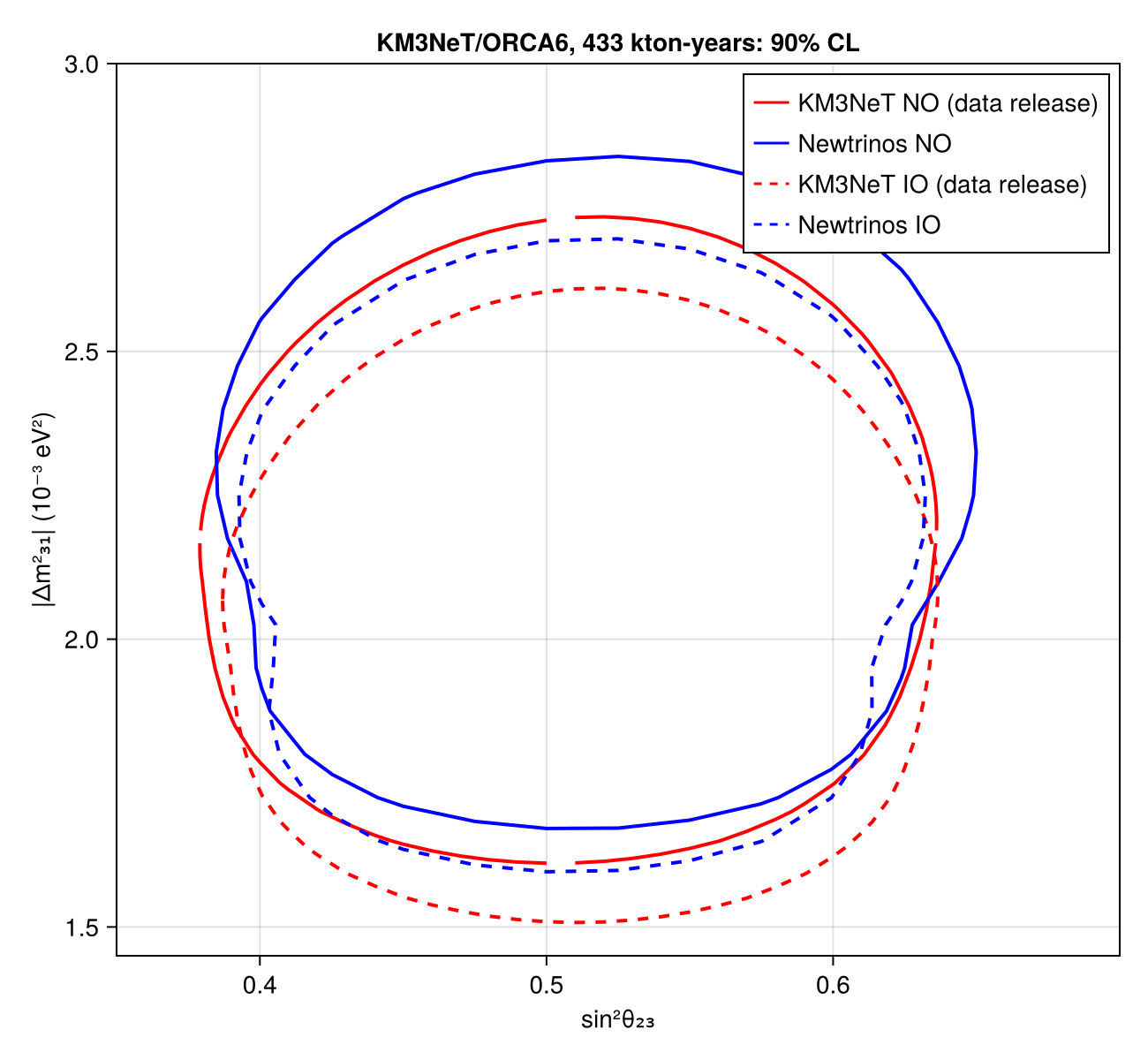
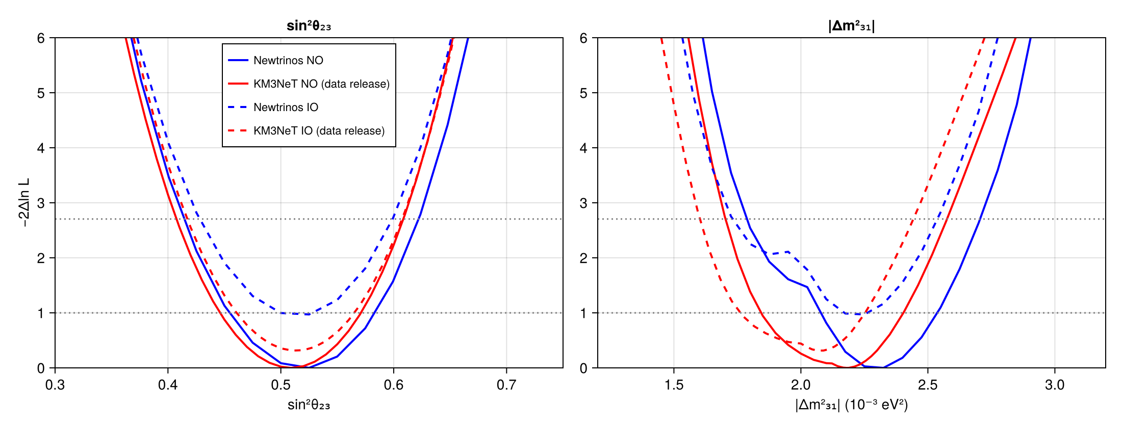
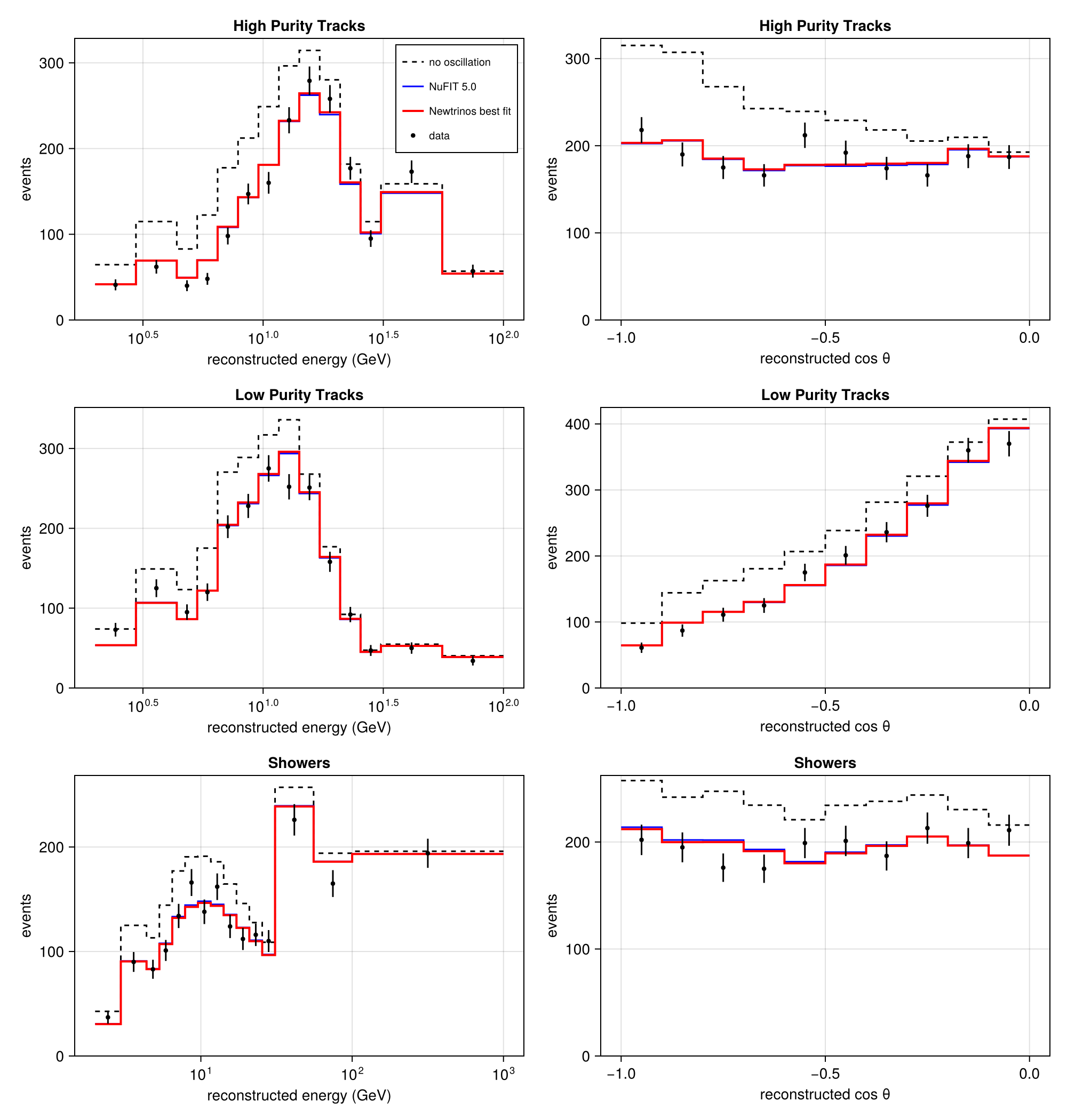
Atmospheric neutrino oscillations with the first six detection units of KM3NeT/ORCA (433 kton-years), using the KM3NeT open-data release of the binned event sample and response, for both mass orderings. Also shown: the 1D profiles of sin²θ₂₃ and |Δm²₃₁| (Fig. 7) against the data-release χ² landscapes, and the event distributions in reconstructed energy and cos θ per event class at the best fit, for NuFIT 5.0 and without oscillation (Fig. 10). In NO, Newtrinos finds sin²θ₂₃ = 0.525 +0.058 −0.070 and |Δm²₃₁| = 2.33 +0.19 −0.25 ×10⁻³ eV² (data release: 0.509 +0.062 −0.063 and 2.18 +0.22 −0.34; paper: 0.51 +0.04 −0.05 and 2.18 +0.25 −0.35), and prefers NO by −2Δln L = 0.97 (KM3NeT: 0.31).
Figures
sin²θ₂₃ – |Δm²₃₁|, 90% CL, NO and IO · Fig. 6 (left)
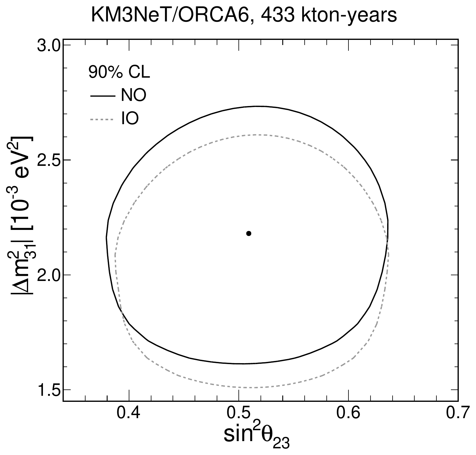
Original figure: KM3NeT, JHEP 10 (2024) 206, Fig. 6 (left), doi:10.1007/JHEP10(2024)206. Not our work; shown for comparison, all rights with the authors and publisher.
1D profiles of sin²θ₂₃ and |Δm²₃₁|, NO and IO, w.r.t. the global minimum: Newtrinos vs data-release χ² landscapes · Fig. 7
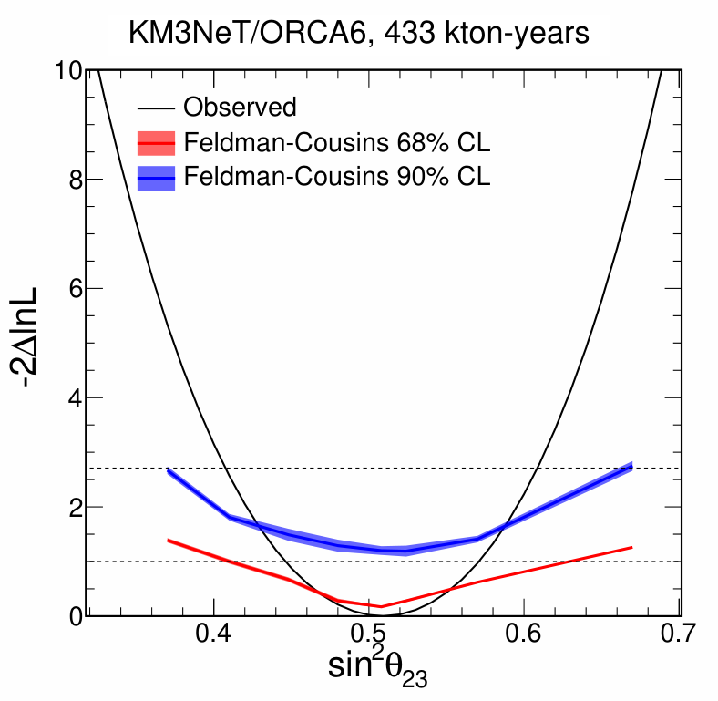
Original figure: KM3NeT, JHEP 10 (2024) 206, Fig. 7, doi:10.1007/JHEP10(2024)206. Not our work; shown for comparison, all rights with the authors and publisher.
Events vs reconstructed energy and cos θ per class: data, Newtrinos best fit, NuFIT 5.0, no oscillation · Fig. 10
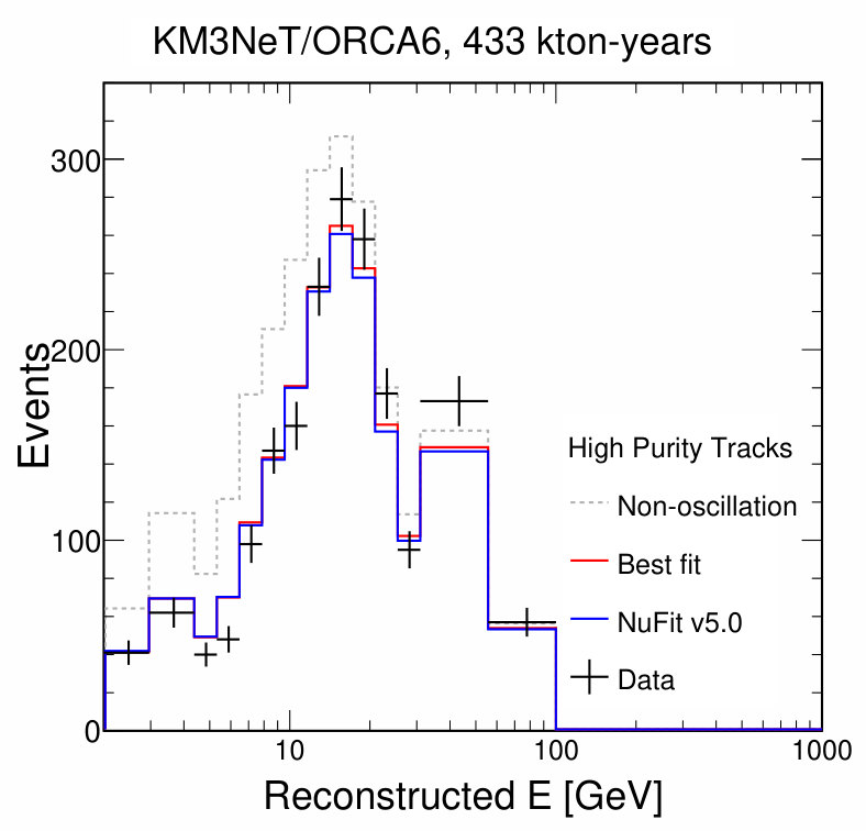
Original figure: KM3NeT, JHEP 10 (2024) 206, Fig. 10, doi:10.1007/JHEP10(2024)206. Not our work; shown for comparison, all rights with the authors and publisher.
Known limitations
- The official contours are computed from the χ² landscapes shipped with the data release; both are shown relative to the minimum over both orderings.
- The energy scale Es is applied as in the paper, as a shift of the true energy of the detector response (flux and oscillation at E/Es, with the Jacobian 1/Es); the flux is the azimuth-averaged Honda 2014 table at Fréjus without mountain, solar minimum, as prescribed by the data release.
- The up/down flux ratio systematic is fixed, as in the Newtrinos validation.
- 1D profiles are the minima over the other parameter of the 21×21 scans and of the data-release landscapes (coarse grids); the paper's Fig. 7 bands from pseudo-experiments are not reproduced. Fig. 10 projects the binned 2D distributions; the no-oscillation and NuFIT 5.0 curves keep the best-fit nuisance parameters, as in the paper.
- Approximate agreement only: our NO region extends further to large sin²θ₂₃ at |Δm²₃₁| ≈ 2.3×10⁻³ eV², and our IO region is narrower in |Δm²₃₁| than the official one.
Reproduce
git clone https://github.com/Newtrinos-org/Newtrinos.jl.git && cd Newtrinos.jl && git checkout 9e58ed6a19- Download reproduce.jl into an empty directory.
julia -t 8 --project=/path/to/Newtrinos.jl reproduce.jl
# Reproduction of KM3NeT, JHEP 10 (2024) 206 [arXiv:2408.07015] with Newtrinos.jl (module `orca`).
# Data: KM3NeT open data, ORCA6 433 kton-years.
# Run from this directory with the Newtrinos.jl environment at the pinned commit:
#   julia -t 8 --project=<path to Newtrinos.jl> reproduce.jl
using Newtrinos, Distributions, DataStructures, Accessors, FileIO, CairoMakie, CSV, DataFrames, DelimitedFiles, Printf

cd(@__DIR__); mkpath("ours"); mkpath("results"); mkpath("cache")
const DATA = joinpath(pkgdir(Newtrinos), "src", "experiments")

# CSV export of a profile scan: one row per grid point, ASCII column names, oscillation parameters in physical
# units (sin²θ, Δm²₃₂ = Δm²₃₁ − Δm²₂₁ in eV², δCP in rad), dchi2 = -2Δlog L w.r.t. `ref` (default: the scan's best fit)
function save_csv(path, r; ref = maximum(r.values.log_posterior))
    ascii(k) = replace(string(k), "θ" => "theta", "Δm²" => "dm2_", "δ" => "d", "₁" => "1", "₂" => "2", "₃" => "3", "CP" => "cp")
    cols = OrderedDict{String,Any}()
    for (k, v) in pairs(r.values)
        x = vec(v)
        if startswith(string(k), "θ")
            cols["sin2_" * ascii(k)] = sin.(x) .^ 2
        elseif k == :Δm²₃₁
            cols["dm2_32"] = x .- vec(r.values.Δm²₂₁)
        end
        cols[ascii(k)] = x
    end
    cols["dchi2"] = 2 .* (ref .- vec(r.values.log_posterior))
    haskey(cols, "llh") && (cols["log_likelihood"] = pop!(cols, "llh"))
    first_cols = filter(in(keys(cols)), ["sin2_theta23", "dm2_32", "dcp", "dchi2", "log_likelihood", "log_posterior"])
    CSV.write(path, DataFrame(cols)[:, vcat(first_cols, setdiff(collect(keys(cols)), first_cols))])
end

# draw each confidence level with its own line style (1σ solid, 2σ dashed, 3σ dotted)
function contours!(ax, res, levels; color, label)
    for (lv, ls) in zip(levels, (:solid, :dash, :dot))
        plot!(ax, res, levels = [lv], color = color, linestyle = ls, label = lv == first(levels) ? label : nothing)
    end
end

experiments = (orca = Newtrinos.orca.configure(),)
likelihood = Newtrinos.generate_likelihood(experiments)
p = Newtrinos.get_params(experiments)
priors = Newtrinos.get_priors(experiments)
priors = merge(priors, (Δm²₂₁ = p.Δm²₂₁, θ₁₂ = p.θ₁₂, δCP = p.δCP, atm_flux_updown_sigma = 0.0,
                        θ₁₃ = Truncated(Normal(0.156, 0.008), 0.13, 0.18), θ₂₃ = Uniform(π / 4 - 0.25, π / 4 + 0.25)))

orderings = (NO = (Δm²₃₁ = (0.0015, 0.003), start = 2.2e-3), IO = (Δm²₃₁ = (-0.003, -0.0015), start = -2.2e-3))
results = map(keys(orderings), values(orderings)) do mo, o
    r = Newtrinos.profile(likelihood, @set(priors.Δm²₃₁ = Uniform(o.Δm²₃₁...)), OrderedDict(:θ₂₃ => 21, :Δm²₃₁ => 21),
                          @set(p.Δm²₃₁ = o.start), cache_dir = "cache/$(mo)")
    mo => r
end |> NamedTuple
global_max = maximum(r -> maximum(r.values.log_posterior), results)
FileIO.save("results/orca6.jld2", Dict(string(k) => v for (k, v) in pairs(results)))
for mo in keys(results)
    save_csv("results/orca6_$(mo)_ssth23_dm31.csv", results[mo]; ref = global_max)
end

# official χ² landscapes of the data release (θ₂₃ in degrees, Δm²₃₁ in eV²), gridded (missing points → NaN)
function official(mo)
    df = CSV.read(joinpath(DATA, "km3net/orca6_433kton/chi2_landscape_$(mo).csv"), DataFrame)
    t = sort(unique(df.theta23)); m = sort(unique(df.dm31))
    χ² = fill(NaN, length(t), length(m))
    for r in eachrow(df)
        χ²[searchsortedfirst(t, r.theta23), searchsortedfirst(m, r.dm31)] = r.chi2
    end
    (ss23 = sind.(t) .^ 2, dm2 = abs.(m) .* 1e3, χ² = χ²)
end
off = (NO = official("NO"), IO = official("IO"))
off_min = minimum(o -> minimum(filter(!isnan, o.χ²)), off)

# Fig. 6 (left): 90% CL, NO and IO
fig = Figure(size = (650, 600))
ax = Axis(fig[1, 1], title = "KM3NeT/ORCA6, 433 kton-years: 90% CL", xlabel = "sin²θ₂₃", ylabel = "|Δm²₃₁| (10⁻³ eV²)")
level = quantile(Chisq(2), 0.9)
for (mo, ls) in ((:NO, :solid), (:IO, :dash))
    o = off[mo]
    contour!(ax, o.ss23, o.dm2, o.χ² .- off_min, levels = [level], color = :red, linestyle = ls, linewidth = 2)
    lines!(ax, [NaN], [NaN], color = :red, linestyle = ls, label = "KM3NeT $(mo) (data release)")
    r = results[mo]
    contour!(ax, sin.(r.axes.θ₂₃) .^ 2, abs.(r.axes.Δm²₃₁) .* 1e3, 2 .* (global_max .- r.values.log_posterior), levels = [level], color = :blue, linestyle = ls, linewidth = 2)
    lines!(ax, [NaN], [NaN], color = :blue, linestyle = ls, label = "Newtrinos $(mo)")
end
xlims!(ax, 0.35, 0.7); ylims!(ax, 1.45, 3.0)
axislegend(ax, position = :rt)
save("ours/contour_NOIO.png", fig)

# ---------------- Fig. 7: 1D profiles of sin²θ₂₃ and |Δm²₃₁| (minimum over the other parameter of the 2D scans) ----------------
"best fit and 1σ range from the Δχ² = 1 crossings (linear interpolation between grid points)"
function onesigma(x, y)
    o = sortperm(x); x = x[o]; y = y[o] .- minimum(y); i = argmin(y)
    j = findlast(>(1), y[1:i]); lo = j === nothing ? x[1] : x[j] + (1 - y[j]) * (x[j+1] - x[j]) / (y[j+1] - y[j])
    j = findfirst(>(1), y[i:end]); hi = j === nothing ? x[end] : (j += i - 1; x[j-1] + (1 - y[j-1]) * (x[j] - x[j-1]) / (y[j] - y[j-1]))
    x[i], hi - x[i], x[i] - lo
end
prof(r, dim) = vec(minimum(2 .* (global_max .- r.values.log_posterior), dims = dim))
oprof(o, dim) = vec(minimum(replace(o.χ², NaN => Inf) .- off_min, dims = dim))
fig = Figure(size = (1100, 420))
ax1 = Axis(fig[1, 1], xlabel = "sin²θ₂₃", ylabel = "−2Δln L", title = "sin²θ₂₃")
ax2 = Axis(fig[1, 2], xlabel = "|Δm²₃₁| (10⁻³ eV²)", title = "|Δm²₃₁|")
open("results/summary.txt", "w") do io
    println(io, "1σ ranges from the 2D scans (Newtrinos | data-release χ² landscape); paper: sin²θ23 = 0.51 +0.04 -0.05, Δm²31 = 2.18 +0.25 -0.35 (NO), [-2.25, -1.76] (IO) ×1e-3 eV², 2 ln(L_NO/L_IO) = 0.31")
    for (mo, ls) in ((:NO, :solid), (:IO, :dash))
        r = results[mo]; o = off[mo]
        s = sin.(r.axes.θ₂₃) .^ 2; m = abs.(r.axes.Δm²₃₁) .* 1e3
        lines!(ax1, s, prof(r, 2), color = :blue, linestyle = ls, linewidth = 2, label = "Newtrinos $mo")
        lines!(ax1, o.ss23, oprof(o, 2), color = :red, linestyle = ls, linewidth = 2, label = "KM3NeT $mo (data release)")
        lines!(ax2, m, prof(r, 1), color = :blue, linestyle = ls, linewidth = 2)
        lines!(ax2, o.dm2, oprof(o, 1), color = :red, linestyle = ls, linewidth = 2)
        @printf(io, "%s: sin2_theta23 %.3f +%.3f -%.3f | %.3f +%.3f -%.3f;  |dm2_31| %.3f +%.3f -%.3f | %.3f +%.3f -%.3f;  min -2ΔlnL %.2f | %.2f\n",
                mo, onesigma(s, prof(r, 2))..., onesigma(o.ss23, oprof(o, 2))..., onesigma(m, prof(r, 1))..., onesigma(o.dm2, oprof(o, 1))...,
                minimum(prof(r, 2)), minimum(oprof(o, 2)))
    end
end
print(read("results/summary.txt", String))
for ax in (ax1, ax2); hlines!(ax, [1.0, quantile(Chisq(1), 0.9)], color = :gray, linestyle = :dot); ylims!(ax, 0, 6); end
xlims!(ax1, 0.3, 0.75); xlims!(ax2, 1.2, 3.2); axislegend(ax1, position = :ct, labelsize = 11)
save("ours/fig7_profiles.png", fig)

# ---------------- Fig. 10: event counts vs reconstructed energy and cos θ, per class, at the global best fit ----------------
mo_bf = argmax(mo -> maximum(results[mo].values.log_posterior), keys(results)); r = results[mo_bf]
ib = argmax(r.values.log_posterior)
bf = merge(p, NamedTuple(k => r.values[k][ib] for k in keys(r.values) if !(k in (:llh, :log_posterior))),
           (θ₂₃ = r.axes.θ₂₃[ib[1]], Δm²₃₁ = r.axes.Δm²₃₁[ib[2]]))
a = experiments.orca.assets; phys = experiments.orca.physics
ex = Newtrinos.orca.get_expected(bf, phys, a)
nufit = merge(bf, (θ₂₃ = asin(sqrt(0.570)), Δm²₃₁ = 2.517e-3, θ₁₃ = asin(sqrt(0.02221))))       # NuFIT 5.0 NO (with SK)
ex_nf = Newtrinos.orca.get_expected(nufit, phys, a)
ex0 = Newtrinos.orca.get_expected(merge(bf, (θ₁₂ = 0.0, θ₁₃ = 0.0, θ₂₃ = 0.0)), phys, a)
bins = a.binning
fig = Figure(size = (1000, 1050))
for (j, (k, name)) in enumerate(((:hpt, "High Purity Tracks"), (:lpt, "Low Purity Tracks"), (:showers, "Showers")))
    d = a.observed[k]; nE = size(d, 1)
    Ee = bins.e_reco_edges[1:nE+1]; ce = bins.cz_reco_edges[1:11]
    for (col, (dim, edges, xl, xs)) in enumerate(((2, Ee, "reconstructed energy (GeV)", log10), (1, ce, "reconstructed cos θ", identity)))
        ax = Axis(fig[j, col], xlabel = xl, ylabel = "events", title = name, xscale = xs)
        proj(h) = vec(sum(h, dims = dim))
        stairs!(ax, edges, vcat(proj(ex0[k]), proj(ex0[k])[end]), step = :post, color = :black, linestyle = :dash, label = "no oscillation")
        stairs!(ax, edges, vcat(proj(ex_nf[k]), proj(ex_nf[k])[end]), step = :post, color = :blue, label = "NuFIT 5.0")
        stairs!(ax, edges, vcat(proj(ex[k]), proj(ex[k])[end]), step = :post, color = :red, linewidth = 2, label = "Newtrinos best fit")
        c = 0.5 .* (edges[1:end-1] .+ edges[2:end]); xs === log10 && (c = sqrt.(edges[1:end-1] .* edges[2:end]))
        errorbars!(ax, c, proj(d), sqrt.(proj(d)), color = :black); scatter!(ax, c, proj(d), color = :black, markersize = 6, label = "data")
        ylims!(ax, 0, nothing)
        j == 1 && col == 1 && axislegend(ax, position = :rt, labelsize = 10)
    end
end
save("ours/fig10_distributions.png", fig)
Provenance
| Newtrinos.jl commit | 9e58ed6a19 (orca) |
|---|---|
| Run date | 2026-10-20T12:34:59Z |
| Wall time | 22.2 min (24 threads) |
| Julia | 1.12.5 |
| Machine | AMD EPYC 7702P 64-Core Processor, 128 hardware threads, Linux |
| Environment | newtrinos_Manifest.toml · run.toml |
Downloads
CSV files hold one row per scan point: the scanned and profiled parameters
(sin2_theta23, dm2_32 in eV², dcp in rad, nuisance parameters), dchi2 = −2Δ log L
and the log-likelihood. JLD2 files contain the full NewtrinosResult objects.
| File | Size | SHA-256 |
|---|---|---|
| ours/contour_NOIO.png | 157.9 kB | f61490b04636… |
| ours/fig10_distributions.png | 243.6 kB | bdaa2c05c4f4… |
| ours/fig7_profiles.png | 189.3 kB | 110b16b7f401… |
| results/orca6.jld2 | 192.9 kB | fe770d7f4e5b… |
| results/orca6_IO_ssth23_dm31.csv | 203.5 kB | 4d9d0ea9faa5… |
| results/orca6_NO_ssth23_dm31.csv | 203.2 kB | bc517c937bb2… |
| results/summary.txt | 474 B | b0e3e55f50b8… |