
NuFIT (Esteban, Gonzalez-Garcia, Maltoni, Martinez-Soler, Pinheiro, Schwetz) · JHEP 12 (2024) 216
NuFit-6.0: updated global analysis of three-flavor neutrino oscillations
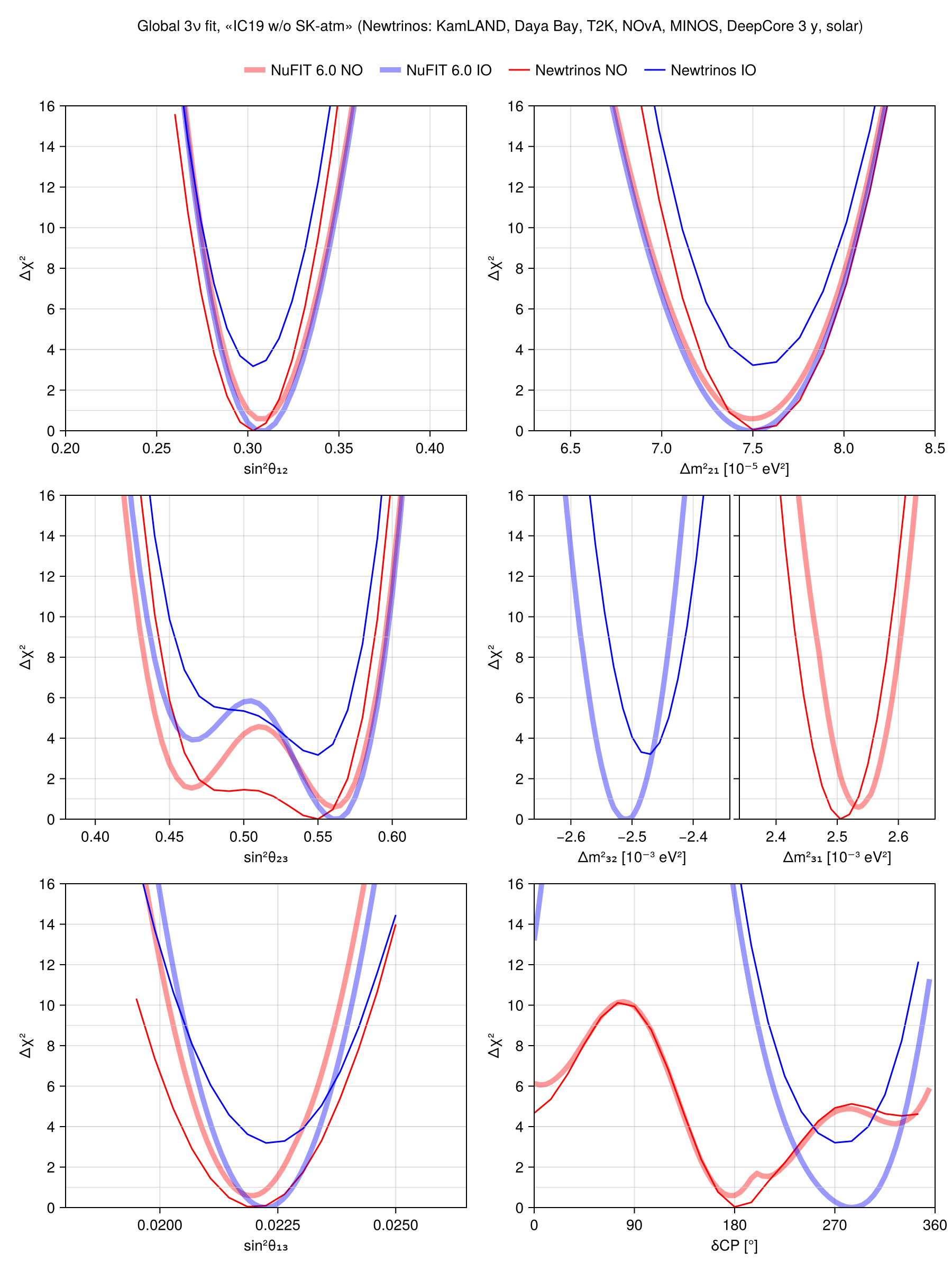
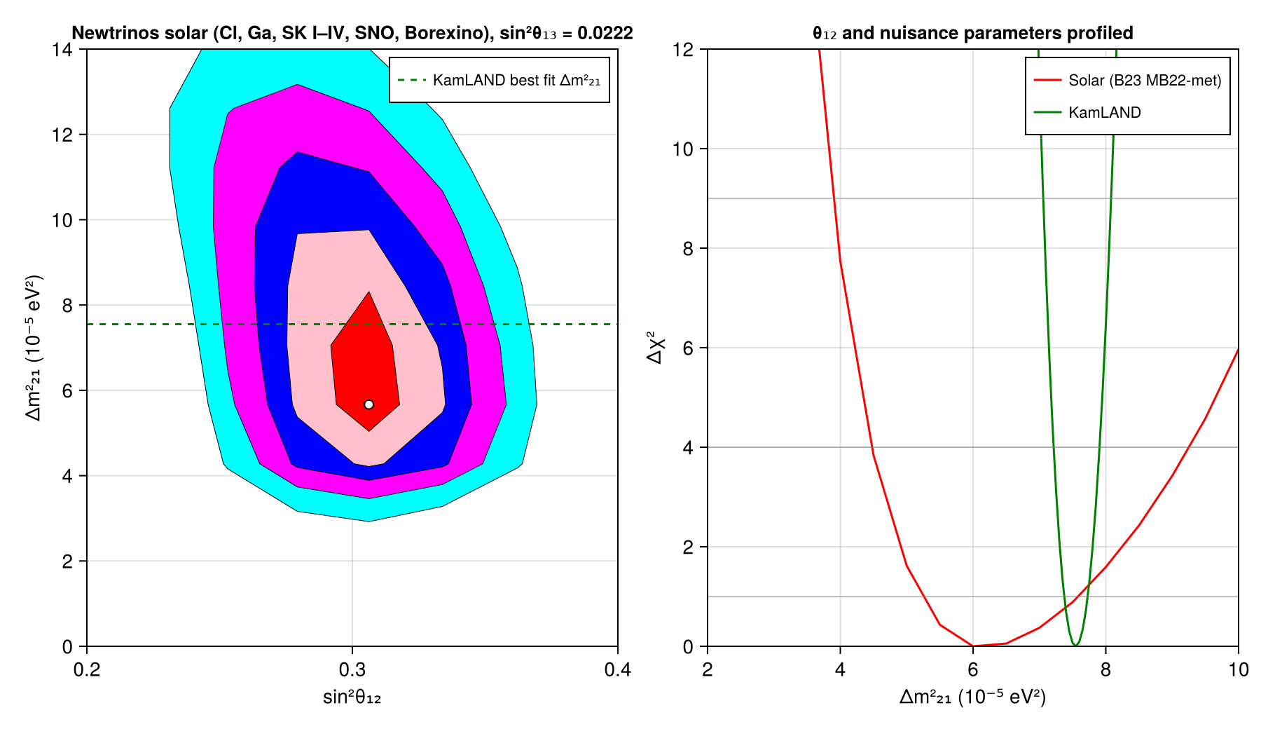
Fig. 1 (global fit, «IC19 w/o SK-atm»): Newtrinos combines KamLAND, Daya Bay, T2K, NOvA, MINOS and IceCube DeepCore (3 years) in full with all solar data, entered as a profiled Δχ² table in (θ₁₂, Δm²₂₁, sin²θ₁₃) (Cl, GALLEX/GNO, SAGE, SNO, SK-I–IV day/night spectra, Borexino Phase I rates, Phase II and III spectral fits). On coarse validation grids the 1D profiles follow NuFIT's: NO best fit sin²θ₁₂ = 0.303, sin²θ₁₃ = 0.0219, sin²θ₂₃ = 0.55, δCP = 180°, Δm²₂₁ = 7.50×10⁻⁵ eV², Δm²₃₁ = 2.505×10⁻³ eV² (NuFIT: 0.310, 0.0219, 0.56, 175°, 7.50, 2.535). The mass ordering preference is reversed: Newtrinos prefers NO by Δχ² ≈ 3.2, NuFIT IO by 0.6. In NO the lower-octant minimum (sin²θ₂₃ ≈ 0.49) is at Δχ² = 1.4 (NuFIT 1.5 w.r.t. its NO minimum). Daya Bay alone has no ordering sensitivity (identical χ² in both orderings); in the global fit it favours NO by 1.75 because ν_μ disappearance fixes |Δm²₃₁| and the implied reactor Δm²ee lies further from Daya Bay's in IO. NOvA adds 1.5 towards NO, T2K 1.0 towards IO (this decomposition is from an earlier run, before the NOvA and T2K audits and the KamLAND update). Fig. 11 (solar vs KamLAND): Solar neutrino determination of θ₁₂ and Δm²₂₁ (sin²θ₁₃ = 0.0222) compared with KamLAND, as in Fig. 11 of NuFIT 6.0. The Newtrinos solar likelihood combines the Homestake, GALLEX/GNO and SAGE rates, the Super-Kamiokande I–IV spectra with the SK-I–IV day/night amplitude fit, the SNO three-phase combination, the Borexino Phase I–II interaction rates and Phase-III spectrum with the B23 MB22-met standard solar model, adiabatic MSW conversion in the Sun and Earth regeneration along PREM chords; solar fluxes, cross sections and detector systematics are profiled. On a coarse validation grid (10×10 in θ₁₂, Δm²₂₁; 17-point Δm²₂₁ profile), Newtrinos finds a solar best fit sin²θ₁₂ = 0.306, Δm²₂₁ = 6.2×10⁻⁵ eV² and Δχ² = 1.0 for the solar data at the KamLAND best fit Δm²₂₁ = 7.55×10⁻⁵ eV² (NuFIT: Δm²₂₁ ≈ 5.7×10⁻⁵ eV², Δχ² ≈ 2.5); with SK's day/night spectra instead of the amplitude fit (earlier run), 6.2×10⁻⁵ eV² and 1.2. The Newtrinos solar region is wider than NuFIT's at 4–5σ.
Figures
Global 3ν fit, «IC19 w/o SK-atm»: 1D Δχ² profiles, NO (red) and IO (blue); NuFIT (thick, from the NuFIT 6.0 tables) vs Newtrinos (thin) · Fig. 1
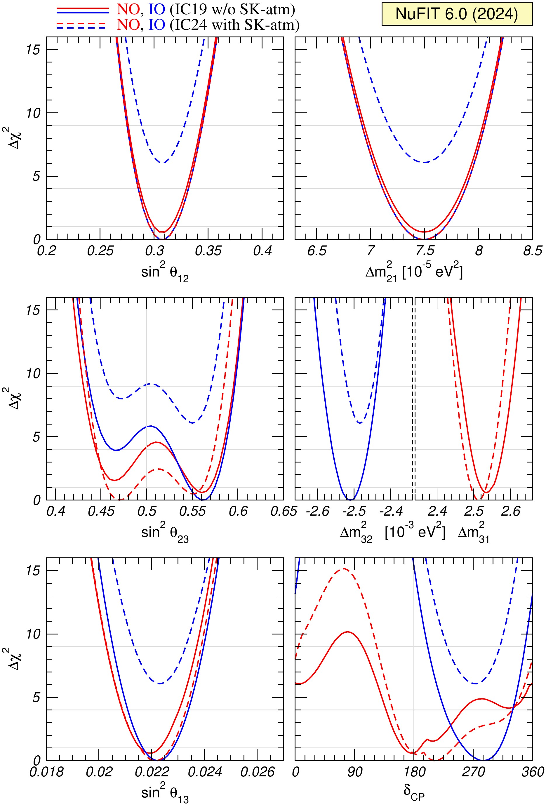
Original figure: NuFIT (Esteban, Gonzalez-Garcia, Maltoni, Martinez-Soler, Pinheiro, Schwetz), JHEP 12 (2024) 216, Fig. 1, doi:10.1007/JHEP12(2024)216. Not our work; shown for comparison, all rights with the authors and publisher.
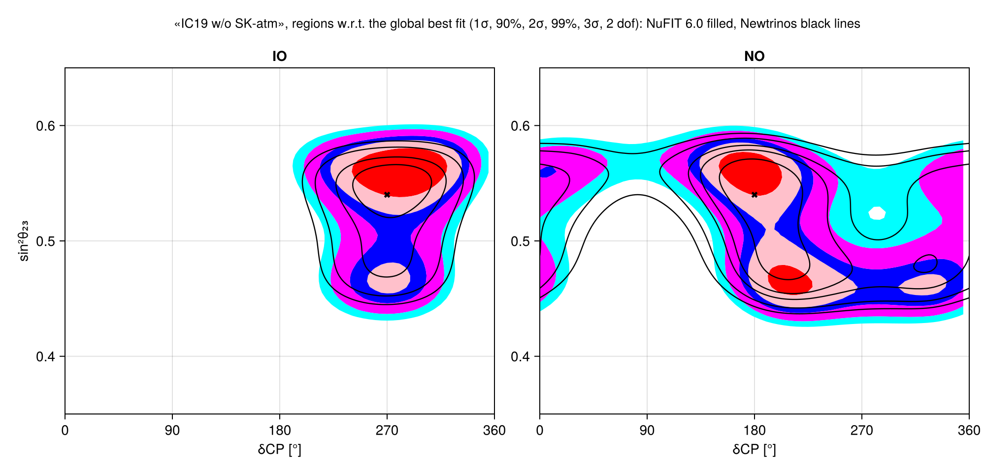
Global 3ν fit, «IC19 w/o SK-atm»: (δCP, sin²θ₂₃) regions for IO and NO w.r.t. the global best fit; NuFIT filled (from the NuFIT 6.0 table), Newtrinos black lines (12×12 grid) · Fig. 8
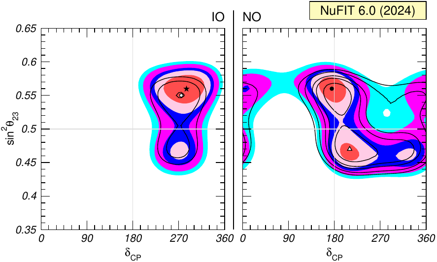
Original figure: NuFIT (Esteban, Gonzalez-Garcia, Maltoni, Martinez-Soler, Pinheiro, Schwetz), JHEP 12 (2024) 216, Fig. 8, doi:10.1007/JHEP12(2024)216. Not our work; shown for comparison, all rights with the authors and publisher.
Solar vs KamLAND: (sin²θ₁₂, Δm²₂₁) regions and Δχ²(Δm²₂₁), sin²θ₁₃ = 0.0222 · Fig. 11
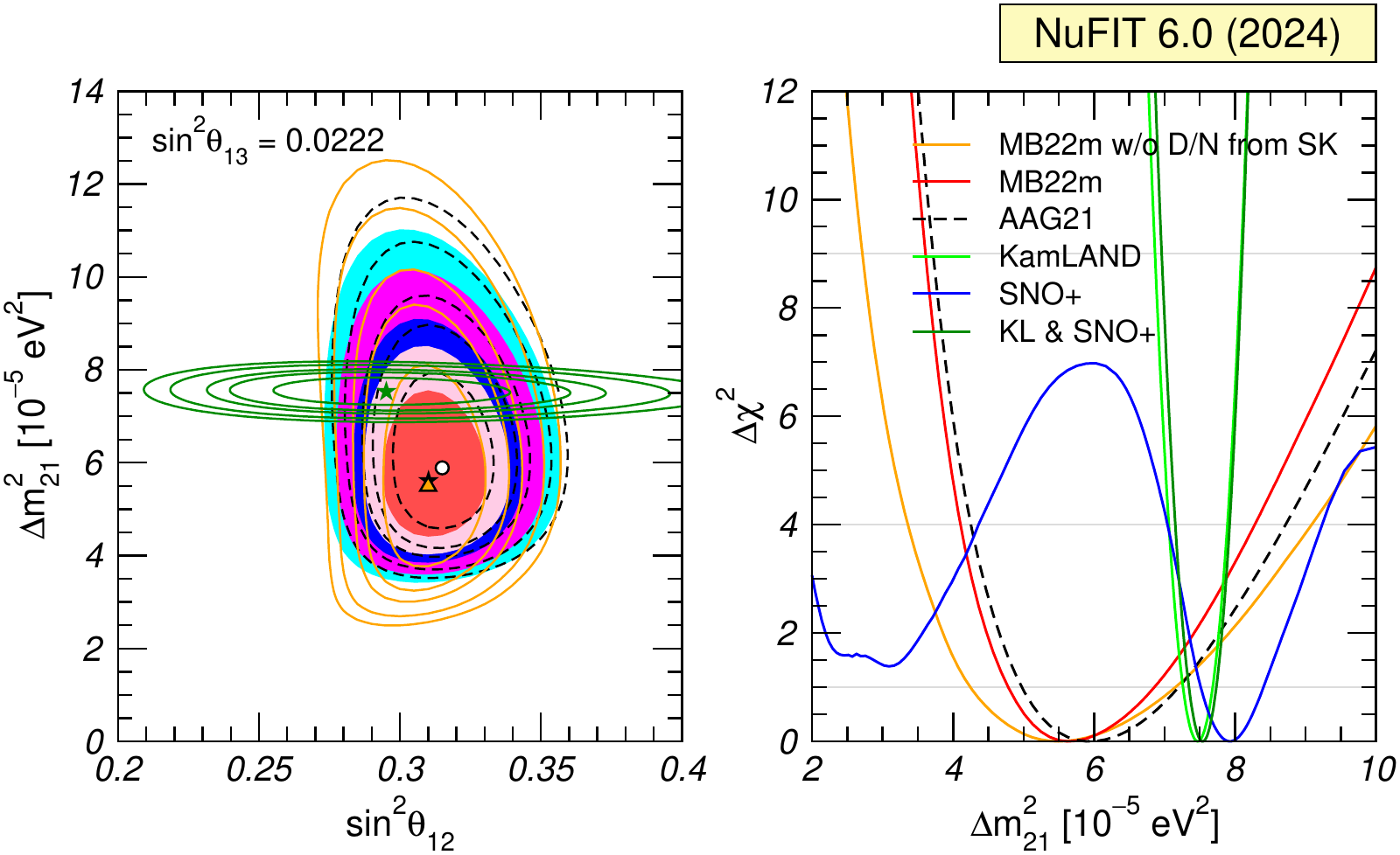
Original figure: NuFIT (Esteban, Gonzalez-Garcia, Maltoni, Martinez-Soler, Pinheiro, Schwetz), JHEP 12 (2024) 216, Fig. 11, doi:10.1007/JHEP12(2024)216. Not our work; shown for comparison, all rights with the authors and publisher.
Known limitations
- Fig. 1: the Newtrinos data set differs from NuFIT's: no RENO, Double Chooz, SNO+ reactor, Super-K atmospheric (not in this variant anyway) or IceCube 2024 data; NOvA, T2K, MINOS and DeepCore as implemented in Newtrinos (data releases and likelihoods may differ from the ones NuFIT uses); Δχ² of both orderings w.r.t. the common best fit, as in NuFIT.
- Fig. 1: coarse validation grids (15–24 points per profile, two starting points each); the solar table is a 15×21×3 grid in (θ₁₂, Δm²₂₁, sin²θ₁₃), interpolated.
- Borexino Phase I and II enter through their published interaction rates (Phase-II correlations as emulated by Super-Kamiokande, arXiv:2312.12907) instead of the 192 Phase-II spectral points used by NuFIT; Phase III enters through a spectral fit of the TFC-subtracted spectrum, with priors on the backgrounds standing in for the non-public tagged spectrum and radial distribution.
- The NuFIT solar analysis details (spectral likelihoods, systematics correlations) are not public; each experiment follows its collaboration's published prescription.
- SK day/night: SK's amplitude fit of the zenith-angle variation (SK-I–IV combined, A_DN vs Δm²₂₁ extracted from PRD 109, 092001, Fig. 52) with the SK spectra merged per energy bin; NuFIT's exact SK day/night treatment is not public.
- Solar flux priors: B23 MB22-met uncertainties and correlations as one multivariate Gaussian.
- KamLAND: the Newtrinos per-period module (2013 data, periods 1–3, reactor fluxes from the IAEA PRIS power histories with Huber–Mueller spectra anchored to Bugey-4; see the KamLAND PRD 88, 033001 entry); NuFIT uses the same three KamLAND periods with Daya Bay reactor fluxes, and SNO+ reactor data, which Newtrinos does not include.
- The AAG21 solar model, the SNO+ and the 'without SK day/night' curves of the original figure are not reproduced.
Reproduce
git clone https://github.com/Newtrinos-org/Newtrinos.jl.git && cd Newtrinos.jl && git checkout c6612c255a- Download reproduce.jl and the
data/folder of this entry into an empty directory. julia -t 8 --project=/path/to/Newtrinos.jl reproduce.jl
# Reproduction of NuFIT 6.0, JHEP 12 (2024) 216 [arXiv:2410.05380], Fig. 11: solar vs KamLAND determination of
# θ₁₂ and Δm²₂₁, with Newtrinos.jl (solar modules `chlorine`, `gallex_gno`, `sage`, `sno`, `sk1_solar`–`sk4_solar`,
# `borexino_ph1`–`borexino_ph3`; `kamland`). Borexino enters through its published interaction rates.
# Run from this directory with the Newtrinos.jl environment at the pinned commit:
#   julia -t 64 --project=<path to Newtrinos.jl> reproduce.jl
using Newtrinos, Distributions, DataStructures, FileIO, CairoMakie, CSV, DataFrames, LinearAlgebra, Interpolations

cd(@__DIR__); mkpath("ours"); mkpath("results"); mkpath("cache")
BLAS.set_num_threads(1)

# CSV export of a profile scan: one row per grid point, ASCII column names, oscillation parameters in physical
# units (sin²θ, Δm² in eV²), dchi2 = -2Δlog L w.r.t. `ref` (default: the scan's best fit)
function save_csv(path, r; ref = maximum(r.values.log_posterior))
    ascii(k) = replace(string(k), "θ" => "theta", "Δm²" => "dm2_", "δ" => "d", "₁" => "1", "₂" => "2", "₃" => "3", "CP" => "cp")
    cols = OrderedDict{String,Any}()
    for (k, v) in pairs(r.values)
        x = vec(v)
        startswith(string(k), "θ") && (cols["sin2_" * ascii(k)] = sin.(x) .^ 2)
        cols[ascii(k)] = x
    end
    cols["dchi2"] = 2 .* (ref .- vec(r.values.log_posterior))
    haskey(cols, "llh") && (cols["log_likelihood"] = pop!(cols, "llh"))
    first_cols = filter(in(keys(cols)), ["sin2_theta12", "dm2_21", "dchi2", "log_likelihood", "log_posterior"])
    CSV.write(path, DataFrame(cols)[:, vcat(first_cols, setdiff(collect(keys(cols)), first_cols))])
end

# NuFIT Fig. 11 conditions: sin²θ₁₃ = 0.0222 fixed; θ₂₃, δCP, Δm²₃₁ irrelevant and fixed; all flux, cross-section and
# detector nuisance parameters profiled with their priors
function setup(experiments)
    p = Newtrinos.get_params(experiments)
    priors = Newtrinos.get_priors(experiments)
    θ13 = asin(sqrt(0.0222))
    p = merge(p, (θ₁₃ = θ13, Δm²₂₁ = 6e-5))
    priors = merge(priors, (θ₁₃ = θ13, θ₂₃ = p.θ₂₃, δCP = p.δCP, Δm²₃₁ = p.Δm²₃₁,
                            θ₁₂ = Uniform(asin(sqrt(0.18)), asin(sqrt(0.42))), Δm²₂₁ = Uniform(1.5e-5, 1.4e-4)))
    Newtrinos.generate_likelihood(experiments), priors, p
end

physics = Newtrinos.solar_common.default_physics()
# SK day/night information from SK's amplitude fit of the zenith-angle variation (SK-I–IV, sk_solar_dn), with the SK
# day/night spectra merged per energy bin
solar = merge(NamedTuple(name => (name in (:sk1_solar, :sk2_solar, :sk3_solar, :sk4_solar) ?
                                  getproperty(Newtrinos, name).configure(physics; daynight = :combined) :
                                  getproperty(Newtrinos, name).configure(physics))
                         for name in (:chlorine, :gallex_gno, :sage, :sno, :sk1_solar, :sk2_solar, :sk3_solar, :sk4_solar,
                                      :borexino_ph1, :borexino_ph2, :borexino_ph3)),
              (sk_solar_dn = Newtrinos.sk_solar_dn.configure(physics; dataset = :sk1to4),))
kamland = (kamland = Newtrinos.kamland.configure(),)

llh, priors, p = setup(solar)
# coarse grids: this entry validates the setup, it does not aim at smooth publication-quality contours
solar_2d = Newtrinos.profile(llh, priors, OrderedDict(:θ₁₂ => 10, :Δm²₂₁ => 10), p, cache_dir = "cache/solar_2d")
priors_dm = merge(priors, (Δm²₂₁ = Uniform(2e-5, 1e-4),))
solar_dm = Newtrinos.profile(llh, priors_dm, OrderedDict(:Δm²₂₁ => 17), p, cache_dir = "cache/solar_dm")
llh, priors, p = setup(kamland)
kamland_dm = Newtrinos.profile(llh, merge(priors, (Δm²₂₁ = Uniform(2e-5, 1e-4),)), OrderedDict(:Δm²₂₁ => 161), merge(p, (Δm²₂₁ = 7.5e-5,)),
                               cache_dir = "cache/kamland_dm")

FileIO.save("results/nufit6_fig11.jld2", Dict("solar_th12_dm21" => solar_2d, "solar_dm21" => solar_dm, "kamland_dm21" => kamland_dm))
save_csv("results/solar_th12_dm21.csv", solar_2d)
save_csv("results/solar_dm21.csv", solar_dm)
save_csv("results/kamland_dm21.csv", kamland_dm)

Δχ²(r) = 2 .* (maximum(r.values.log_posterior) .- r.values.log_posterior)

fig = Figure(size = (900, 520))
# left: solar regions, 1σ–5σ (2 dof), and KamLAND best fit
ax = Axis(fig[1, 1], title = "Newtrinos solar (Cl, Ga, SK I–IV, SNO, Borexino), sin²θ₁₃ = 0.0222",
          xlabel = "sin²θ₁₂", ylabel = "Δm²₂₁ (10⁻⁵ eV²)", titlesize = 13)
x = sin.(solar_2d.axes.θ₁₂) .^ 2; y = solar_2d.axes.Δm²₂₁ .* 1e5
levels = [quantile(Chisq(2), 1 - 2 * ccdf(Normal(), n)) for n in 1:5]
contourf!(ax, x, y, Δχ²(solar_2d), levels = vcat(0, levels), colormap = [:red, :pink, :blue, :magenta, :cyan])
contour!(ax, x, y, Δχ²(solar_2d), levels = levels, color = :black, linewidth = 0.5)
i = argmax(solar_2d.values.log_posterior)
scatter!(ax, [x[i[1]]], [y[i[2]]], color = :white, strokecolor = :black, strokewidth = 1)
kl_best = kamland_dm.axes.Δm²₂₁[argmax(kamland_dm.values.log_posterior)]
hlines!(ax, [kl_best * 1e5], color = :green, linestyle = :dash, label = "KamLAND best fit Δm²₂₁")
xlims!(ax, 0.2, 0.4); ylims!(ax, 0, 14)
axislegend(ax, position = :rt, labelsize = 11)
# right: Δχ²(Δm²₂₁), θ₁₂ profiled
ax2 = Axis(fig[1, 2], xlabel = "Δm²₂₁ (10⁻⁵ eV²)", ylabel = "Δχ²", title = "θ₁₂ and nuisance parameters profiled", titlesize = 13)
lines!(ax2, solar_dm.axes.Δm²₂₁ .* 1e5, Δχ²(solar_dm), color = :red, label = "Solar (B23 MB22-met)")
lines!(ax2, kamland_dm.axes.Δm²₂₁ .* 1e5, Δχ²(kamland_dm), color = :green, label = "KamLAND")
hlines!(ax2, [1, 4, 9], color = :gray, linewidth = 0.5)
xlims!(ax2, 2, 10); ylims!(ax2, 0, 12)
axislegend(ax2, position = :rt, labelsize = 11)
save("ours/fig11_solar_kamland.png", fig)

# key numbers for the summary
# cubic spline through the coarse 1D solar profile
dm_ax = range(first(solar_dm.axes.Δm²₂₁), last(solar_dm.axes.Δm²₂₁), length = length(solar_dm.axes.Δm²₂₁))
@assert collect(dm_ax) ≈ solar_dm.axes.Δm²₂₁
χ²_solar = cubic_spline_interpolation(dm_ax, Δχ²(solar_dm))
dm_fine = range(first(dm_ax), last(dm_ax), length = 2001)
best = dm_fine[argmin(χ²_solar.(dm_fine))]
at_kl = χ²_solar(kl_best) - minimum(χ²_solar.(dm_fine))
open("results/summary.txt", "w") do io
    println(io, "solar best-fit sin2_theta12 = ", round(x[i[1]], digits = 3), ", dm2_21 = ", round(y[i[2]], digits = 2), "e-5 eV^2 (2D grid)")
    println(io, "solar best-fit dm2_21 (1D profile) = ", round(best * 1e5, digits = 2), "e-5 eV^2")
    println(io, "KamLAND best-fit dm2_21 = ", round(kl_best * 1e5, digits = 2), "e-5 eV^2")
    println(io, "solar dchi2 at the KamLAND best fit = ", round(at_kl, digits = 2))
end
print(read("results/summary.txt", String))

# ═══════════════════════════════════════════════════════════════════════════════════════════════════════════════════
# Fig. 1: global 3ν fit, variant «IC19 w/o SK-atm». Newtrinos approximation of the NuFIT data set: KamLAND, Daya Bay,
# T2K, NOvA, MINOS and IceCube DeepCore 3 y in full, plus all solar data as a profiled Δχ² table in
# (θ₁₂, Δm²₂₁, sin²θ₁₃). 1D profiles of the six oscillation parameters for each ordering, every point minimised over all
# other parameters from two starting points (θ₂₃ octants; δCP for the θ₂₃ profile). The fits run on NPROC worker
# processes × NTHR threads (env, default 24 × 5).
using Distributed, Printf
const NPROC = parse(Int, get(ENV, "NPROC", "24")); const NTHR = parse(Int, get(ENV, "NTHR", "5"))
"Run `f` over `jobs` in batches of NTHR (threads within a worker), on NPROC freshly started workers set up by `init`."
function distributed_fits(init, jobs)
    ws = addprocs(NPROC; exeflags = `-t $NTHR --project=$(Base.active_project())`)
    try
        Distributed.remotecall_eval(Main, ws, init)
        batches = [jobs[i:min(i + NTHR - 1, end)] for i in 1:NTHR:length(jobs)]
        reduce(vcat, pmap(b -> Main.fit_batch(b), WorkerPool(ws), batches))
    finally
        rmprocs(ws)
    end
end
const ENTRY = @__DIR__

# solar Δχ² table: Cl, GALLEX/GNO, SAGE, SNO, SK-I–IV (day/night spectra), Borexino Phase I (rates), Phase II
# (spectral fit), Phase III; solar nuisance parameters profiled; θ₂₃, δCP, Δm²₃₁ irrelevant and fixed
solar_init = quote
    using Newtrinos, Distributions, LinearAlgebra
    using BAT: distprod
    BLAS.set_num_threads(1)
    const sp = Newtrinos.solar_common.default_physics()
    const solar = (chlorine = Newtrinos.chlorine.configure(sp), gallex_gno = Newtrinos.gallex_gno.configure(sp),
                   sage = Newtrinos.sage.configure(sp), sno = Newtrinos.sno.configure(sp), sk_solar = Newtrinos.sk_solar.configure(sp),
                   borexino_ph1 = Newtrinos.borexino_ph1.configure(sp),
                   borexino_ph2_spectrum = Newtrinos.borexino_ph2_spectrum.configure(sp),
                   borexino_ph3 = Newtrinos.borexino_ph3.configure(sp))
    const LLH = Newtrinos.generate_likelihood(solar)
    const P0 = merge(Newtrinos.get_params(solar), (θ₂₃ = asin(sqrt(0.47)), δCP = 3.70, Δm²₃₁ = 2.513e-3))
    const PR0 = merge(Newtrinos.get_priors(solar), (θ₂₃ = P0.θ₂₃, δCP = P0.δCP, Δm²₃₁ = P0.Δm²₃₁))
    function fit_point(θ12, dm21, θ13)
        p = merge(P0, (θ₁₂ = θ12, Δm²₂₁ = dm21, θ₁₃ = θ13))
        pr = merge(PR0, (θ₁₂ = θ12, Δm²₂₁ = dm21, θ₁₃ = θ13))
        Newtrinos.find_mle_cached(LLH, distprod(; pr...), p, joinpath($ENTRY, "cache", "solar_table");
                                  adsel = Newtrinos.ADTypes.AutoForwardDiff())[2]
    end
    fit_batch(pts) = (out = Vector{Float64}(undef, length(pts)); Threads.@threads for i in eachindex(pts); out[i] = fit_point(pts[i]...); end; out)
end
θ12_tab = collect(range(asin(sqrt(0.20)), asin(sqrt(0.42)), length = 15))
dm21_tab = collect(range(4.0e-5, 11.0e-5, length = 21))
pts = vec([(a, b, asin(sqrt(c))) for a in θ12_tab, b in dm21_tab, c in [0.0195, 0.0222, 0.0249]])
mkpath("cache/solar_table")
lp_solar = distributed_fits(solar_init, pts)
CSV.write("results/solar_table.csv", DataFrame(sin2_theta12 = [sin(p[1])^2 for p in pts], dm2_21 = [p[2] for p in pts],
                                               sin2_theta13 = [sin(p[3])^2 for p in pts], minus2lnL = -2 .* lp_solar))

global_init = quote
    using Newtrinos, Distributions, LinearAlgebra, CSV, DataFrames
    using BAT: distprod
    BLAS.set_num_threads(1)
    "Solar Δχ² table as a chi2map experiment, interpolated in (θ₁₂, Δm²₂₁, sin²θ₁₃)."
    function solar_term(file)
        df = CSV.read(file, DataFrame)
        θ = sort(unique(asin.(sqrt.(df.sin2_theta12)))); dm = sort(unique(df.dm2_21)); s13 = sort(unique(df.sin2_theta13))
        tab = fill(NaN, length(θ), length(dm), length(s13))
        for r in eachrow(df)
            tab[searchsortedfirst(θ, asin(sqrt(r.sin2_theta12)) - 1e-12), searchsortedfirst(dm, r.dm2_21 - 1e-20),
                searchsortedfirst(s13, r.sin2_theta13 - 1e-12)] = r.minus2lnL
        end
        @assert !any(isnan, tab)
        ax = (range(θ[1], θ[end], length = length(θ)), range(dm[1], dm[end], length = length(dm)), range(s13[1], s13[end], length = length(s13)))
        Newtrinos.chi2map.configure((p -> p.θ₁₂, p -> p.Δm²₂₁, p -> sin(p.θ₁₃)^2), ax, tab; title = "solar (all data, profiled)")
    end
    "Experiments, likelihood, start parameters and priors (flat in θ, δCP, Δm²) for one mass ordering."
    function setup(ordering)
        exps = (kamland = Newtrinos.kamland.configure(), dayabay = Newtrinos.dayabay.configure(),
                t2k = Newtrinos.t2k.configure(), nova = Newtrinos.nova.configure(), minos = Newtrinos.minos.configure(),
                deepcore_3y = Newtrinos.deepcore_3y.configure(), solar = solar_term(joinpath($ENTRY, "results", "solar_table.csv")))
        p = Newtrinos.get_params(exps)
        pr = Newtrinos.get_priors(exps)
        if ordering == :NO
            p = merge(p, (Δm²₃₁ = 2.51e-3,)); pr = merge(pr, (Δm²₃₁ = Uniform(2.2e-3, 2.9e-3),))
        else
            p = merge(p, (Δm²₃₁ = -2.41e-3,)); pr = merge(pr, (Δm²₃₁ = Uniform(-2.8e-3, -2.1e-3),))
        end
        p = merge(p, (θ₁₂ = asin(sqrt(0.307)), θ₁₃ = asin(sqrt(0.0222)), θ₂₃ = asin(sqrt(0.5)), δCP = 3.7, Δm²₂₁ = 7.5e-5))
        pr = merge(pr, (θ₁₂ = Uniform(asin(sqrt(0.24)), asin(sqrt(0.38))), θ₁₃ = Uniform(asin(sqrt(0.018)), asin(sqrt(0.026))),
                        θ₂₃ = Uniform(asin(sqrt(0.35)), asin(sqrt(0.65))), δCP = Uniform(0, 2π), Δm²₂₁ = Uniform(6.0e-5, 9.0e-5)))
        (; exps, llh = Newtrinos.generate_likelihood(exps), p, pr)
    end
    const SETUPS = Dict(o => setup(o) for o in (:NO, :IO))
    "Profile log likelihood with `var` fixed to `val`: the log posterior minus the (constant) flat oscillation priors."
    function fit_point(ordering, var, val, start)
        s = SETUPS[ordering]
        p = merge(s.p, start, NamedTuple{(var,)}((val,)))
        pr = merge(s.pr, NamedTuple{(var,)}((val,)))
        r = Newtrinos.find_mle_cached(s.llh, distprod(; pr...), p, joinpath($ENTRY, "cache", "global");
                                      adsel = Newtrinos.ADTypes.AutoForwardDiff())
        r[2] - sum(logpdf(pr[k], r[3][k]) for k in (:θ₁₂, :θ₁₃, :θ₂₃, :δCP, :Δm²₂₁, :Δm²₃₁) if k != var)
    end
    fit_batch(jobs) = (out = Vector{Float64}(undef, length(jobs)); Threads.@threads for i in eachindex(jobs); out[i] = fit_point(jobs[i]...); end; out)
end
s2θ(x) = asin(sqrt(x))
function grid(ordering)
    dm3l = ordering == :NO ? range(2.40e-3, 2.64e-3, length = 17) : range(-2.62e-3, -2.38e-3, length = 17) .+ 7.5e-5   # Δm²₃₁ (IO: Δm²₃₂ + Δm²₂₁)
    (θ₁₂ = s2θ.(range(0.26, 0.36, length = 15)), θ₁₃ = s2θ.(range(0.0195, 0.0250, length = 15)),
     θ₂₃ = s2θ.(range(0.40, 0.62, length = 23)), δCP = deg2rad.(0:15:345), Δm²₂₁ = range(6.6e-5, 8.4e-5, length = 15),
     Δm²₃₁ = dm3l)
end
starts(var) = var == :θ₂₃ ? [(δCP = 3.4,), (δCP = 4.7,)] : [(θ₂₃ = s2θ(0.45),), (θ₂₃ = s2θ(0.57),)]
jobs = [(o, var, v, st) for o in (:NO, :IO) for var in keys(grid(o)) for v in grid(o)[var] for st in starts(var)]
mkpath("cache/global")
lp_global = distributed_fits(global_init, jobs)
raw = DataFrame(ordering = [string(j[1]) for j in jobs], var = [string(j[2]) for j in jobs], value = [j[3] for j in jobs],
                log_likelihood = lp_global)
prof = combine(groupby(raw, [:ordering, :var, :value]), :log_likelihood => maximum => :log_likelihood)
prof.dchi2 = 2 .* (maximum(prof.log_likelihood) .- prof.log_likelihood)    # w.r.t. the best fit of both orderings
# plotted quantities as in NuFIT: sin²θ, δCP in degrees, Δm²₂₁ in 10⁻⁵ eV², Δm²₃₁ (NO) and Δm²₃₂ (IO) in 10⁻³ eV²
# (Δm²₃₂ = Δm²₃₁ − Δm²₂₁ with Δm²₂₁ = 7.5×10⁻⁵ eV²; the shift from the fitted Δm²₂₁ is < 10⁻⁶ eV²)
xplot(var, o, v) = var == "Δm²₃₁" ? (o == "NO" ? v : v - 7.5e-5) * 1e3 : var == "δCP" ? rad2deg(v) :
                   var == "Δm²₂₁" ? v * 1e5 : sin(v)^2
prof.x = [xplot(r.var, r.ordering, r.value) for r in eachrow(prof)]
sort!(prof, [:ordering, :var, :x])
CSV.write("results/global_profiles.csv", prof[:, [:ordering, :var, :x, :dchi2, :log_likelihood]])

tag = Dict("θ₁₂" => "T12", "θ₁₃" => "T13", "θ₂₃" => "T23", "δCP" => "DCP", "Δm²₂₁" => "DMS", "Δm²₃₁" => "DMA")
function nufit(o, var)
    t = CSV.read("data/nufit6_TBoff/TBoff_$(o)_$(tag[var]).csv", DataFrame)
    x = var == "Δm²₂₁" ? 10 .^ t.c0 .* 1e5 : var == "δCP" ? mod.(t.c0, 360) : t.c0
    k = sortperm(x); x, y = x[k], t.c1[k]
    k = unique(i -> x[i], eachindex(x)); x[k], y[k]               # δCP: 0° and 360° both tabulated
end
ours(o, var) = (d = prof[(prof.ordering .== o) .& (prof.var .== var), :]; (d.x, d.dchi2))

# layout of NuFIT Fig. 1
fig = Figure(size = (900, 1200))
panels = [("θ₁₂", 1, 1, "sin²θ₁₂", (0.2, 0.42)), ("Δm²₂₁", 1, 2, "Δm²₂₁ [10⁻⁵ eV²]", (6.3, 8.5)),
          ("θ₂₃", 2, 1, "sin²θ₂₃", (0.38, 0.65)), ("θ₁₃", 3, 1, "sin²θ₁₃", (0.018, 0.0265)), ("δCP", 3, 2, "δCP [°]", (0, 360))]
style(o) = o == "NO" ? :red : :blue
for (var, r, c, lab, xr) in panels
    ax = Axis(fig[r, c], xlabel = lab, ylabel = "Δχ²")
    for o in ("NO", "IO")
        lines!(ax, nufit(o, var)..., color = (style(o), 0.4), linewidth = 5)
        lines!(ax, ours(o, var)..., color = style(o), linewidth = 1.5)
    end
    var == "δCP" && (ax.xticks = 0:90:360)
    hlines!(ax, [1, 4, 9], color = :gray80, linewidth = 0.5); xlims!(ax, xr...); ylims!(ax, 0, 16)
end
g = fig[2, 2] = GridLayout()
for (k, o, xr, lab) in ((1, "IO", (-2.66, -2.34), "Δm²₃₂ [10⁻³ eV²]"), (2, "NO", (2.34, 2.66), "Δm²₃₁ [10⁻³ eV²]"))
    ax = Axis(g[1, k], xlabel = lab, ylabel = k == 1 ? "Δχ²" : "", yticklabelsvisible = k == 1)
    lines!(ax, nufit(o, "Δm²₃₁")..., color = (style(o), 0.4), linewidth = 5)
    lines!(ax, ours(o, "Δm²₃₁")..., color = style(o), linewidth = 1.5)
    hlines!(ax, [1, 4, 9], color = :gray80, linewidth = 0.5); xlims!(ax, xr...); ylims!(ax, 0, 16)
end
colgap!(g, 4)
Legend(fig[0, :], [LineElement(color = (:red, 0.4), linewidth = 5), LineElement(color = (:blue, 0.4), linewidth = 5),
                   LineElement(color = :red, linewidth = 1.5), LineElement(color = :blue, linewidth = 1.5)],
       ["NuFIT 6.0 NO", "NuFIT 6.0 IO", "Newtrinos NO", "Newtrinos IO"], orientation = :horizontal, framevisible = false)
Label(fig[-1, :], "Global 3ν fit, «IC19 w/o SK-atm» (Newtrinos: KamLAND, Daya Bay, T2K, NOvA, MINOS, DeepCore 3 y, solar)", fontsize = 14)
save("ours/fig1_global_profiles.png", fig)

# best fits and 1σ ranges (Δχ² = 1 w.r.t. each ordering's minimum), as in NuFIT Table 1
function onesigma(x, y)
    m = minimum(y); itp = linear_interpolation(x, y .- m)
    fine = range(first(x), last(x), length = 4001); inside = fine[itp.(fine) .<= 1]
    x[argmin(y)], first(inside), last(inside), m
end
open("results/summary_global.txt", "w") do io
    println(io, "best fit [1σ range] (Δχ² of the ordering's minimum); Newtrinos | NuFIT 6.0 IC19 w/o SK-atm")
    for var in ("θ₁₂", "θ₁₃", "θ₂₃", "δCP", "Δm²₂₁", "Δm²₃₁"), o in ("NO", "IO")
        f(t) = @sprintf("%.4g [%.4g, %.4g] (%.2f)", t...)
        println(io, rpad("$(tag[var]) $o", 8), rpad(f(onesigma(ours(o, var)...)), 40), "| ", f(onesigma(nufit(o, var)...)))
    end
end
print(read("results/summary_global.txt", String))

# ═══════════════════════════════════════════════════════════════════════════════════════════════════════════════════
# Fig. 8: (δCP, sin²θ₂₃) regions for IO and NO w.r.t. the global best fit, all other parameters profiled (same global
# fit as Fig. 1); coarse 12 × 12 grid per ordering
dcp_2d = deg2rad.(0:30:330); s23_2d = range(0.40, 0.62, length = 12)
jobs2d = [(o, (δCP = d, θ₂₃ = s2θ(s)), nothing) for o in (:NO, :IO) for s in s23_2d for d in dcp_2d]
fit2d_init = quote
    $global_init
    "Profile log likelihood with θ₂₃ and δCP fixed."
    function fit_point(ordering, fixed, _)
        s = SETUPS[ordering]
        r = Newtrinos.find_mle_cached(s.llh, distprod(; merge(s.pr, fixed)...), merge(s.p, fixed), joinpath($ENTRY, "cache", "global_2d");
                                      adsel = Newtrinos.ADTypes.AutoForwardDiff())
        r[2] - sum(logpdf(s.pr[k], r[3][k]) for k in (:θ₁₂, :θ₁₃, :Δm²₂₁, :Δm²₃₁))
    end
end
mkpath("cache/global_2d")
lp2d = distributed_fits(fit2d_init, jobs2d)
gbest = max(maximum(prof.log_likelihood), maximum(lp2d))
CSV.write("results/global_dcp_th23.csv", DataFrame(ordering = [string(j[1]) for j in jobs2d], sin2_theta23 = [sin(j[2].θ₂₃)^2 for j in jobs2d],
                                                   dcp_deg = [rad2deg(j[2].δCP) for j in jobs2d], dchi2 = 2 .* (gbest .- lp2d)))

levels2 = [2.30, 4.61, 6.18, 9.21, 11.83]        # 1σ, 90 %, 2σ, 99 %, 3σ (2 dof)
fig = Figure(size = (1000, 480))
for (k, o) in enumerate(("IO", "NO"))
    ax = Axis(fig[1, k], xlabel = "δCP [°]", ylabel = k == 1 ? "sin²θ₂₃" : "", title = o, xticks = 0:90:360)
    # NuFIT: filled regions from the 2D table (δCP −180…180 → 0…360)
    t = CSV.read("data/nufit6_TBoff/TBoff_$(o)_T23_DCP.csv", DataFrame)
    sx = sort(unique(t.c0)); dx = sort(unique(mod.(t.c1, 360)))
    z = fill(NaN, length(dx), length(sx))
    for r in eachrow(t); z[searchsortedfirst(dx, mod(r.c1, 360)), searchsortedfirst(sx, r.c0)] = r.c2; end
    contourf!(ax, dx, sx, z, levels = vcat(0, levels2), colormap = [:red, :pink, :blue, :magenta, :cyan])
    # Newtrinos: contours of the coarse grid, bicubic in (δCP periodic, sin²θ₂₃)
    zn = [2 * (gbest - lp2d[findfirst(j -> j[1] == Symbol(o) && j[2].δCP == d && j[2].θ₂₃ == s2θ(s), jobs2d)]) for d in dcp_2d, s in s23_2d]
    itp = cubic_spline_interpolation((range(0, 2π, length = 13), s23_2d), vcat(zn, zn[1:1, :]))
    df = range(0, 2π, length = 181); sf = range(first(s23_2d), last(s23_2d), length = 111)
    contour!(ax, rad2deg.(df), sf, [itp(a, b) for a in df, b in sf], levels = levels2, color = :black, linewidth = 1.2)
    i = argmin(zn); scatter!(ax, [rad2deg(dcp_2d[i[1]])], [s23_2d[i[2]]], color = :black, marker = :xcross)
    xlims!(ax, 0, 360); ylims!(ax, 0.35, 0.65)
end
Label(fig[0, :], "«IC19 w/o SK-atm», regions w.r.t. the global best fit (1σ, 90%, 2σ, 99%, 3σ, 2 dof): NuFIT 6.0 filled, Newtrinos black lines", fontsize = 13)
save("ours/fig8_dcp_th23.png", fig)
Provenance
| Newtrinos.jl commit | c6612c255a (solar_flux, solar_xsec, solar_common, chlorine, gallex_gno, sage, sno, sk_solar_common, sk1_solar, sk2_solar, sk3_solar, sk4_solar, sk_solar, borexino_ph1, borexino_ph2, borexino_ph2_spectrum, borexino_ph3, kamland, reactor_flux, dayabay, t2k, nova, minos, deepcore_3y, chi2map) |
|---|---|
| Run date | 2026-10-22T07:22:57Z |
| Wall time | 135.5 min (128 threads), 1616 of 1947 fit points reused from an earlier run at the same commit |
| Julia | 1.12.5 |
| Machine | AMD EPYC 7702P 64-Core Processor, 128 hardware threads, Linux |
| Environment | newtrinos_Manifest.toml · run.toml |
Downloads
CSV files hold one row per scan point: the scanned and profiled parameters
(sin2_theta23, dm2_32 in eV², dcp in rad, nuisance parameters), dchi2 = −2Δ log L
and the log-likelihood. JLD2 files contain the full NewtrinosResult objects.
| File | Size | SHA-256 |
|---|---|---|
| ours/fig11_solar_kamland.png | 181.3 kB | df61f73ce194… |
| ours/fig1_global_profiles.png | 523.5 kB | 28547b6d61ae… |
| ours/fig8_dcp_th23.png | 246.3 kB | d3e7f88674ee… |
| results/global_dcp_th23.csv | 12.6 kB | c8eb7e2e3148… |
| results/global_profiles.csv | 13.6 kB | 9c308dac4eb7… |
| results/kamland_dm21.csv | 53.2 kB | 1bd4e18278b4… |
| results/nufit6_fig11.jld2 | 187.6 kB | d2b3150c75f6… |
| results/solar_dm21.csv | 14.6 kB | 8a0566632fba… |
| results/solar_table.csv | 57.0 kB | 126e70b1ee56… |
| results/solar_th12_dm21.csv | 83.4 kB | 2c5f9c4f8426… |
| results/summary.txt | 201 B | a659904b64d0… |
| results/summary_global.txt | 1.0 kB | ec3230ff470f… |