
A. Strumia, F. Vissani · Phys. Lett. B 564, 42 (2003)
Precise quasielastic neutrino/nucleon cross section
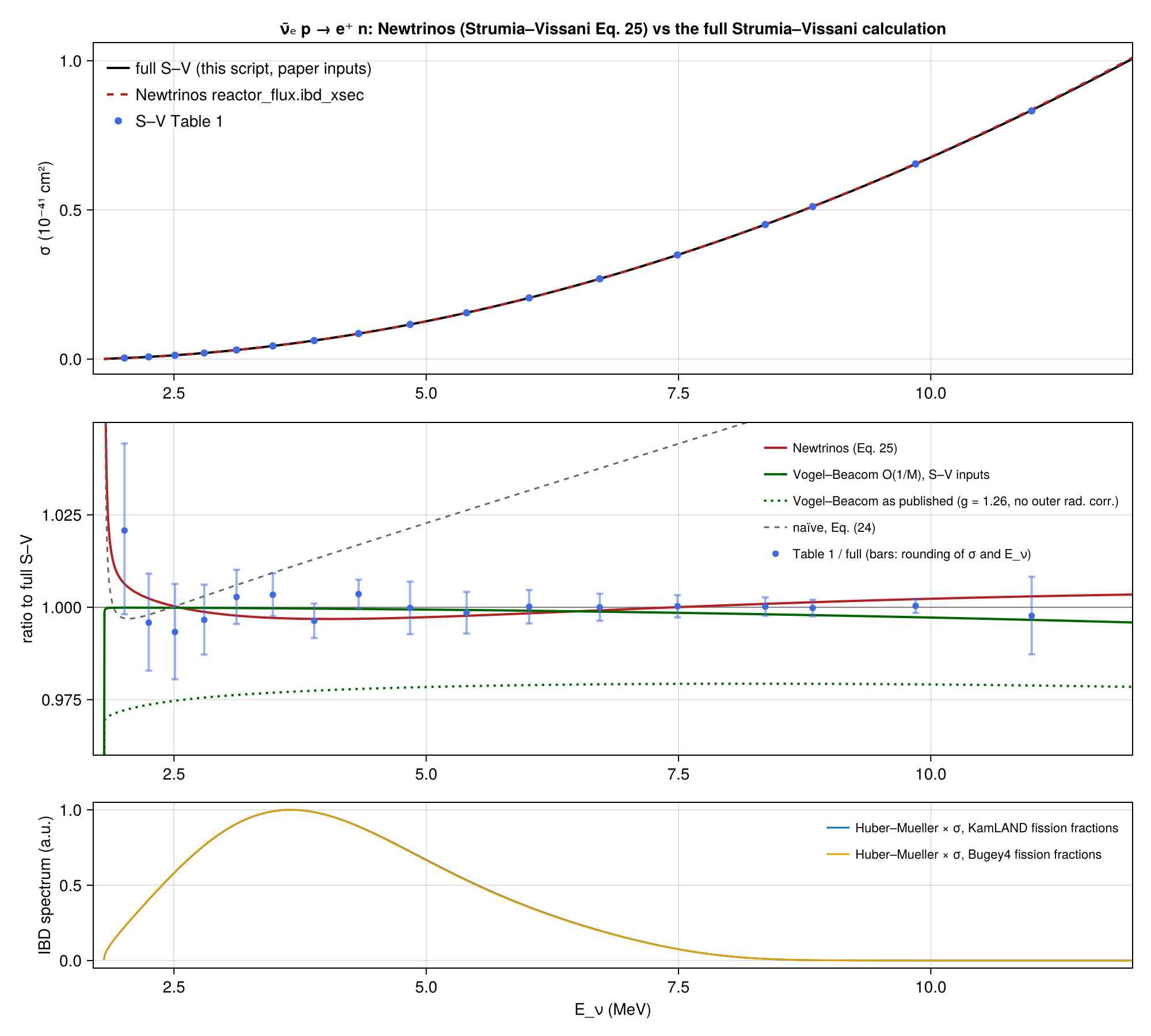
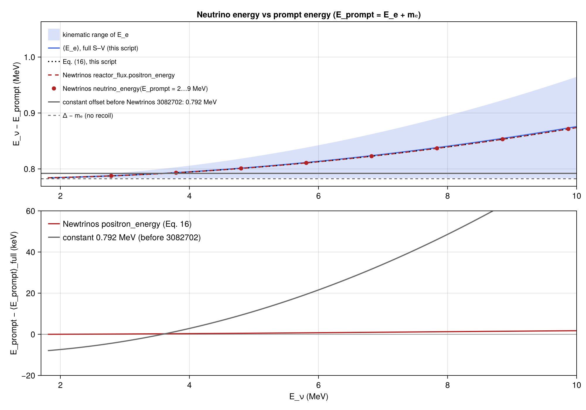
The inverse-beta-decay cross section used by Newtrinos' reactor_flux module (the approximation of Strumia & Vissani, Eq. 25) compared with the full Strumia–Vissani calculation, implemented here from the paper's Eqs. (3)–(14) with its inputs, and with the O(1/M) result of Vogel & Beacom (PRD 60, 053003). The implementation reproduces Table 1 within its rounding for all rows up to 40 MeV (σ in 41 of 44 rows, ⟨E_e⟩ in 43), and Table 2's comparison of Eq. (25) and of Vogel–Beacom. At reactor energies Newtrinos' cross section is within 0.35 % of the full one between 2.2 and 10 MeV (+0.7 % at 2 MeV, where Eq. 25 has the zeroth-order threshold); the IBD yield per fission of the Huber–Mueller spectra is 0.19 % below the full calculation for KamLAND's and Bugey-4's fission fractions. Vogel–Beacom with the same inputs agrees with the full result to 0.1 % below 6 MeV. Also shown: the relation between neutrino and prompt energy including the neutron recoil. This comparison led to a change in Newtrinos (3082702): the KamLAND module now maps prompt to neutrino energy with reactor_flux.positron_energy/neutrino_energy (Eq. 16), which agree with the mean positron energy of the full calculation to within 1.7 keV below 10 MeV, instead of a constant offset of 0.792 MeV.
Figures
σ(ν̄ₑ p → e⁺ n) at reactor energies: Newtrinos (Eq. 25), the full Strumia–Vissani calculation, Table 1, Vogel–Beacom and the naïve formula; ratios to the full result, with the Huber–Mueller IBD spectrum · Table 1
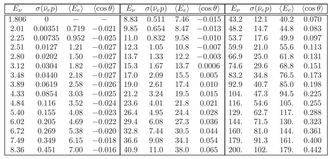
Original figure: A. Strumia, F. Vissani, Phys. Lett. B 564, 42 (2003), Table 1, doi:10.1016/S0370-2693(03)00616-6. Not our work; shown for comparison, all rights with the authors and publisher.
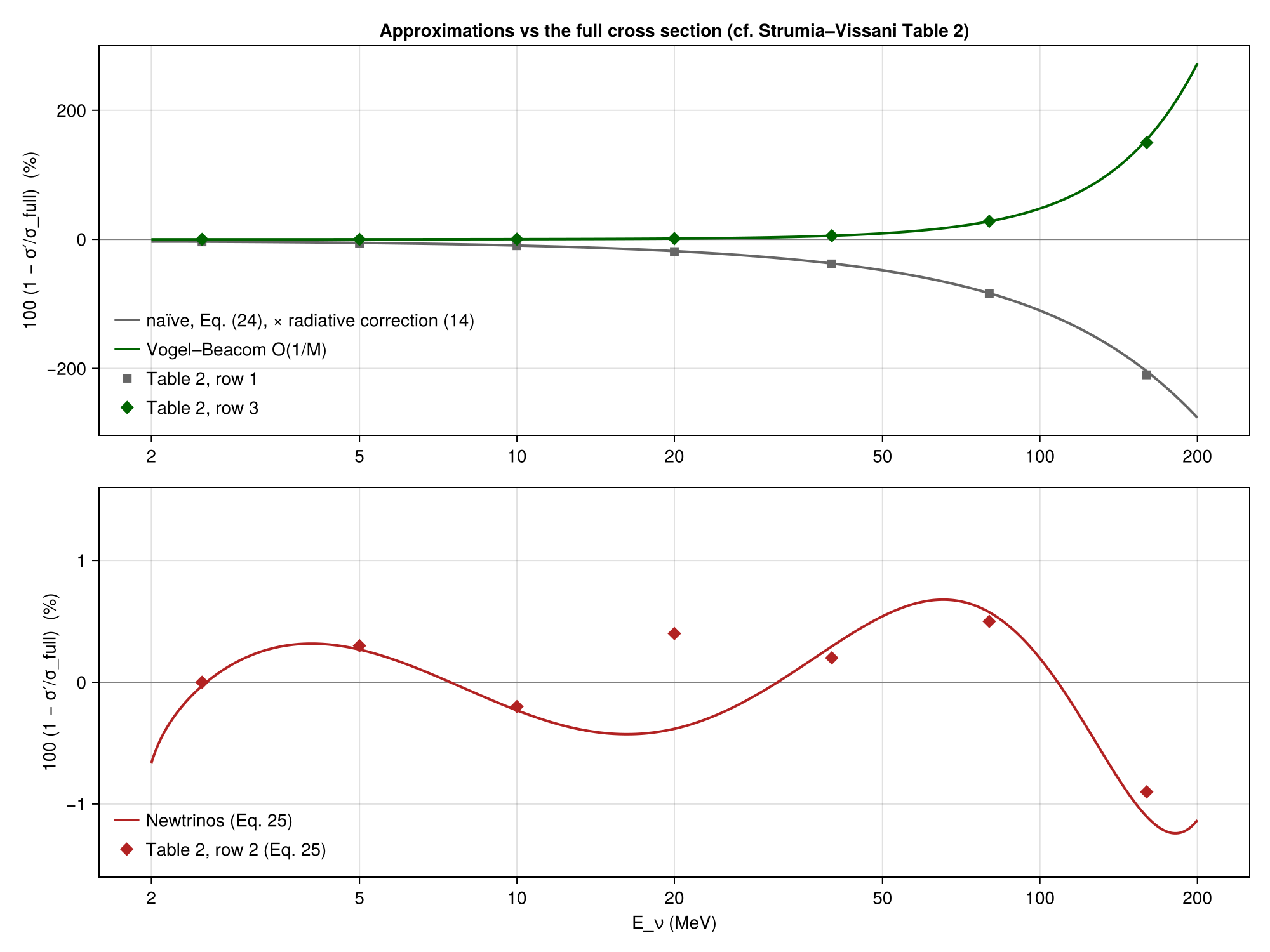
Approximations vs the full cross section, 2–200 MeV: naïve Eq. (24), Vogel–Beacom O(1/M) and Newtrinos' Eq. (25), with the values of Table 2 · Table 2
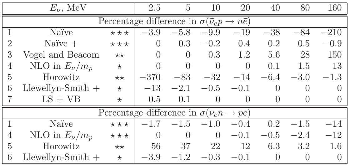
Original figure: A. Strumia, F. Vissani, Phys. Lett. B 564, 42 (2003), Table 2, doi:10.1016/S0370-2693(03)00616-6. Not our work; shown for comparison, all rights with the authors and publisher.
E_ν − E_prompt with the neutron recoil: full ⟨E_e⟩, Eq. (16), Newtrinos' positron_energy / neutrino_energy (since 3082702) and the constant offset used before; prompt-energy differences to the full calculation · Eq. (16)
Eq. (16)
Known limitations
- The 'full' curve is this entry's implementation of the paper's Eqs. (3)–(7), (11)–(14) (form factors of Eq. (7), radiative correction of Eq. (14), the paper's G_F, cos θ_C = 0.9746, g₁(0) = −1.270, M_A² = 1 GeV², PDG 2002 masses). It agrees with Table 1 within the rounding of σ and E_ν at all energies up to 40 MeV; above 40 MeV σ is up to 0.9 % and ⟨cos θ⟩ up to 0.005 off (σ outside the rounding at 144–179 MeV), probably from an input detail of the paper that is not stated; this does not affect reactor energies.
- Table 2, row 1 (naïve Eq. 24) is reproduced to 0.3–0.8 points up to 80 MeV (5 points at 160 MeV) only when Eq. (24) is also given the radiative correction of Eq. (14); row 2 (Eq. 25) is reproduced at all energies except 20 MeV, where the paper quotes +0.4 % and we find −0.4 % (possibly a sign misprint; the neighbouring values match); row 3 (Vogel–Beacom, evaluated with the Strumia–Vissani inputs and radiative correction) is reproduced to 0.2 points up to 80 MeV and to 5 points at 160 MeV.
- Normalisation: the paper's inputs correspond to |V_ud|²(1 + 3λ²) = 5.546, i.e. a neutron lifetime of 885.1 s (with τn |V_ud|²(1 + 3λ²) = 4908.6 s, Czarnecki, Marciano & Sirlin 2018). With today's values the cross section is 0.76 % larger (PDG 2024 τn = 878.4 s) or 0.51 % larger (PDG 2024 V_ud and λ). Newtrinos (pinned commit) uses the paper's normalisation unchanged. This has no effect on the KamLAND module, whose rate is anchored to the Bugey-4 measured yield per fission computed with the same cross section (the scale cancels to 10⁻⁴); it would matter for any prediction of absolute IBD rates.
- Vogel–Beacom as published (f = 1, g = 1.26, cos θ_C = 0.974, inner radiative correction 2.4 %, no outer radiative correction) is 2.1–2.8 % below the full Strumia–Vissani cross section at reactor energies; the difference is entirely due to the inputs and the outer radiative correction, not to the O(1/M) expansion.
- Prompt energy (E_prompt = E_e + mₑ): before Newtrinos 3082702 the KamLAND module used E_ν = E_prompt + 0.792 MeV at all energies. With the neutron recoil, E_ν − ⟨E_prompt⟩ grows from 0.784 MeV at threshold to 0.803 MeV at E_ν = 5 MeV and 0.841 MeV at 8 MeV (0.798 MeV averaged over the KamLAND spectrum), so the constant put prompt energies up to 50 keV (0.7 %) too high at the upper end of the spectrum and 8 keV too low near threshold (within KamLAND's 1.8 % energy-scale uncertainty). Since 3082702 (the pinned commit) the prediction integrates over E_ν(E_prompt) from
reactor_flux.neutrino_energywith the Jacobian; ΔE_NU is kept only for plots. Effect on KamLAND: no-oscillation shape χ² against KamLAND's published expectation 1.67 → 1.63 (17 bins), log-likelihood at the default point −143.632 → −144.639, grid best fit with nuisances fixed Δm²₂₁ 7.675 → 7.70 ×10⁻⁵ eV² (+0.3 %). Results of KamLAND entries run at earlier commits use the constant offset. The spread of E_e at fixed E_ν (blue band) is far below the detector resolution. - Only ν̄ₑ p is checked; ⟨cos θ⟩ and νₑ n are not used by Newtrinos. Huber–Mueller spectra are used here only as weights (they are the subject of a separate entry).
Reproduce
git clone https://github.com/Newtrinos-org/Newtrinos.jl.git && cd Newtrinos.jl && git checkout 3082702195- Download reproduce.jl and the
data/folder of this entry into an empty directory. julia -t 8 --project=/path/to/Newtrinos.jl reproduce.jl
# Verification of the Newtrinos.jl inverse-beta-decay cross section (module `reactor_flux`, `ibd_xsec`: Strumia & Vissani,
# Eq. (25)) against the full calculation of A. Strumia and F. Vissani, Phys. Lett. B 564, 42 (2003) (their Tables 1 and 2),
# and against the O(1/M) result of P. Vogel and J. F. Beacom, Phys. Rev. D 60, 053003 (1999).
# Run from this directory with the Newtrinos.jl environment at the pinned commit:
#   julia --project=<path to Newtrinos.jl> reproduce.jl
using Newtrinos, CairoMakie, DelimitedFiles, LinearAlgebra, Printf

cd(@__DIR__); mkpath("ours"); mkpath("results")

const RF = Newtrinos.reactor_flux

# ------------------------------------------------------------------------------------------------
# Full Strumia–Vissani cross section, Eqs. (3)–(7), (11)–(14), with the paper's inputs
# ------------------------------------------------------------------------------------------------
const mn, mp, me = 939.56536, 938.27203, 0.510998902        # MeV (PDG 2002, as in the paper)
const Δ, M = mn - mp, (mn + mp) / 2
const GF, COS_C, G1_0 = 1.16637e-11, 0.9746, -1.270         # MeV⁻², cos θ_C, g₁(0)
const MV2, MA2, ξ, mπ = 0.71e6, 1.0e6, 3.706, 139.57        # MeV², MeV², κp − κn, MeV
const α = 1 / 137.035999
const HBARC2 = 3.893794e-22                                 # (ħc)² [MeV² cm²]
const δ = (mn^2 - mp^2 - me^2) / (2mp)
const E_THR = ((mn + me)^2 - mp^2) / (2mp)

function gauss_legendre(n)
    F = eigen(SymTridiagonal(zeros(n), [i / sqrt(4i^2 - 1) for i in 1:n-1]))
    F.values, 2 .* F.vectors[1, :] .^ 2
end
const GL = gauss_legendre(64)
integrate(f, a, b) = (h = (b - a) / 2; c = (a + b) / 2; h * sum(w * f(c + h * x) for (x, w) in zip(GL...)))

"|M|² of Eq. (5)–(7) (averaged over initial, summed over final polarisations)."
function M2(s, t, u)
    f1 = (1 - (1 + ξ) * t / (4M^2)) / ((1 - t / (4M^2)) * (1 - t / MV2)^2)
    f2 = ξ / ((1 - t / (4M^2)) * (1 - t / MV2)^2)
    g1 = G1_0 / (1 - t / MA2)^2
    g2 = 2 * M^2 * g1 / (mπ^2 - t)
    m2 = me^2
    A = ((t - m2) * (4 * f1^2 * (4 * M^2 + t + m2) + 4 * g1^2 * (-4 * M^2 + t + m2) + f2^2 * (t^2 / M^2 + 4 * t + 4 * m2) +
                     4 * m2 * t * g2^2 / M^2 + 8 * f1 * f2 * (2 * t + m2) + 16 * m2 * g1 * g2) -
         Δ^2 * ((4 * f1^2 + t * f2^2 / M^2) * (4 * M^2 + t - m2) + 4 * g1^2 * (4 * M^2 - t + m2) + 4 * m2 * g2^2 * (t - m2) / M^2 +
                8 * f1 * f2 * (2 * t - m2) + 16 * m2 * g1 * g2) - 32 * m2 * M * Δ * g1 * (f1 + f2)) / 16
    B = (16 * t * g1 * (f1 + f2) + 4 * m2 * Δ * (f2^2 + f1 * f2 + 2 * g1 * g2) / M) / 16
    C = (4 * (f1^2 + g1^2) - t * f2^2 / M^2) / 16
    su = s - u
    A - su * B + su^2 * C
end

"Radiative correction of Eq. (14) (Kurylov, Ramsey-Musolf, Vogel)."
radcorr(Ee) = 1 + α / π * (6.00 + 1.5 * log(mp / (2Ee)) + 1.2 * (me / Ee)^1.5)

"dσ/dE_e [cm² / MeV], Eq. (11)."
function dσdEe(Eν, Ee; rc = true)
    s = mp^2 + 2mp * Eν; t = mn^2 - mp^2 - 2mp * (Eν - Ee); su = 2mp * (Eν + Ee) - me^2
    GF^2 * COS_C^2 / (2π * (s - mp^2)^2) * M2(s, t, s - su) * 2mp * HBARC2 * (rc ? radcorr(Ee) : 1.0)
end

"Positron energy range E₁ ≤ E_e ≤ E₂, Eqs. (12)–(13)."
function ee_range(Eν)
    s = mp^2 + 2mp * Eν; rs = sqrt(s)
    EνCM = (s - mp^2) / (2rs); EeCM = (s - mn^2 + me^2) / (2rs)
    peCM = sqrt(max((s - (mn - me)^2) * (s - (mn + me)^2), 0.0)) / (2rs)
    (Eν - δ - EνCM * (EeCM + peCM) / mp, Eν - δ - EνCM * (EeCM - peCM) / mp)
end

"Total σ [cm²], ⟨E_e⟩ [MeV] and ⟨cos θ⟩ of the full calculation."
function sv_full(Eν; rc = true)
    Eν <= E_THR && return (σ = 0.0, Ee = NaN, cosθ = NaN)
    E1, E2 = ee_range(Eν)
    w(Ee) = dσdEe(Eν, Ee; rc)
    σ = integrate(w, E1, E2)
    cosθ(Ee) = (t = mn^2 - mp^2 - 2mp * (Eν - Ee); (t - me^2 + 2Eν * Ee) / (2Eν * sqrt(Ee^2 - me^2)))
    (σ = σ, Ee = integrate(e -> e * w(e), E1, E2) / σ, cosθ = integrate(e -> cosθ(e) * w(e), E1, E2) / σ)
end

"⟨E_e⟩ ≈ (E₁ + E₂)/2, Eq. (16)."
ee_eq16(Eν) = sum(ee_range(Eν)) / 2

"Naïve cross section, Eq. (24) [cm²]."
σ_naive(Eν) = (Ee = Eν - Δ; Ee > me ? 9.52e-44 * sqrt(Ee^2 - me^2) * Ee : 0.0)

"""
Vogel–Beacom O(1/M) total cross section, Eqs. (9), (13)–(15), integrated over cos θ. `inputs = :sv` uses the couplings of
Strumia–Vissani and their radiative correction (the comparison of their Table 2); `inputs = :vb` the published ones
(f = 1, g = 1.26, cos θ_C = 0.974, Δ_inner = 0.024, no outer radiative correction).
"""
function σ_vb(Eν; inputs = :sv)
    f, f2 = 1.0, ξ
    g, cc, inner, rc = inputs == :sv ? (-G1_0, COS_C, 0.0, true) : (1.26, 0.974, 0.024, false)
    Ee0 = Eν - Δ
    Ee0 <= me && return 0.0
    σ0 = GF^2 * cc^2 / π * (1 + inner) * HBARC2
    pe0 = sqrt(Ee0^2 - me^2); ve0 = pe0 / Ee0; y2 = (Δ^2 - me^2) / 2
    integrate(-1.0, 1.0) do c
        Ee1 = Ee0 * (1 - Eν / M * (1 - ve0 * c)) - y2 / M
        pe1 = sqrt(max(Ee1^2 - me^2, 0.0)); ve1 = pe1 / Ee1
        Γ = 2 * (f + f2) * g * ((2Ee0 + Δ) * (1 - ve0 * c) - me^2 / Ee0) + (f^2 + g^2) * (Δ * (1 + ve0 * c) + me^2 / Ee0) +
            (f^2 + 3g^2) * ((Ee0 + Δ) * (1 - c / ve0) - Δ) + (f^2 - g^2) * ((Ee0 + Δ) * (1 - c / ve0) - Δ) * ve0 * c
        (σ0 / 2 * ((f^2 + 3g^2) + (f^2 - g^2) * ve1 * c) * Ee1 * pe1 - σ0 / 2 * Γ / M * Ee0 * pe0) * (rc ? radcorr(Ee1) : 1.0)
    end
end

σ_nt(Eν) = RF.ibd_xsec(Eν)        # Newtrinos

# ------------------------------------------------------------------------------------------------
# 1. Table 1: σ, ⟨E_e⟩, ⟨cos θ⟩ — within the rounding of the table (including the rounding of E_ν)
# ------------------------------------------------------------------------------------------------
halfunit(s) = (s = strip(s); occursin('.', s) ? 0.5 * 10.0^(-length(split(s, '.')[2])) : 0.5)
raw = readdlm("data/sv_table1.csv", ',', String; comments = true, comment_char = '#')[2:end, :]
tab1 = parse.(Float64, raw)
io = open("results/table1.csv", "w")
println(io, "E_nu,sigma_paper_1e-41cm2,sigma_full_1e-41cm2,sigma_newtrinos_1e-41cm2,sigma_full_range_lo,sigma_full_range_hi,sigma_consistent,",
        "Ee_paper,Ee_full,Ee_consistent,cos_paper,cos_full,cos_consistent")
n_ok = zeros(Int, 3)
t1 = map(1:size(tab1, 1)) do i
    E = tab1[i, 1]; hE = halfunit(raw[i, 1])
    f = sv_full(E); lo, hi = sv_full(E - hE), sv_full(E + hE)
    rng(x, xl, xh) = (min(x, xl, xh), max(x, xl, xh))
    sr = rng(f.σ, lo.σ, hi.σ) ./ 1e-41; er = rng(f.Ee, lo.Ee, hi.Ee); cr = rng(f.cosθ, lo.cosθ, hi.cosθ)
    ok(r, v, h) = r[1] - 1e-12 <= v + h && r[2] + 1e-12 >= v - h
    oks = (ok(sr, tab1[i, 2], halfunit(raw[i, 2])), ok(er, tab1[i, 3], halfunit(raw[i, 3])), ok(cr, tab1[i, 4], halfunit(raw[i, 4])))
    n_ok .+= oks
    println(io, join(Any[E, tab1[i, 2], f.σ / 1e-41, σ_nt(E) / 1e-41, sr..., oks[1], tab1[i, 3], f.Ee, oks[2], tab1[i, 4], f.cosθ, oks[3]], ","))
    (E = E, hE = hE, σ = tab1[i, 2], hσ = halfunit(raw[i, 2]), full = f.σ / 1e-41, sr = sr)
end
close(io)
@printf "Table 1 (44 rows) consistent within rounding: σ %d, ⟨E_e⟩ %d, ⟨cos θ⟩ %d\n" n_ok...

# ------------------------------------------------------------------------------------------------
# 2. Table 2: percentage differences 100 (1 − σ'/σ) of the approximations
# ------------------------------------------------------------------------------------------------
t2 = readdlm("data/sv_table2.csv", ',', Float64; comments = true, header = true)[1]
pct(σ′, σ) = 100 * (1 - σ′ / σ)
io = open("results/table2.csv", "w")
println(io, "E_nu,naive_paper,naive_ours_rc_on_eq24,eq25_paper,eq25_ours,newtrinos_ours,vb_paper,vb_ours")
println("\nTable 2 (paper / ours):")
for r in eachrow(t2)
    E = r[1]; F = sv_full(E).σ
    # the paper's naïve row is reproduced when eq. (24) also carries the radiative correction of eq. (14) (see caveats)
    nv = pct(σ_naive(E) * radcorr(E - Δ), F)
    vals = (nv, pct(1e-43 * sqrt((E - Δ)^2 - me^2) * (E - Δ) * E^(-0.07056 + 0.02018log(E) - 0.001953log(E)^3), F), pct(σ_nt(E), F), pct(σ_vb(E), F))
    @printf "  %5.1f MeV  naïve %6.1f / %6.1f   Eq. (25) %5.1f / %5.2f  (Newtrinos %5.2f)   VB %5.1f / %5.1f\n" E r[2] vals[1] r[3] vals[2] vals[3] r[4] vals[4]
    println(io, join([E, r[2], vals[1], r[3], vals[2], vals[3], r[4], vals[4]], ","))
end
close(io)

# ------------------------------------------------------------------------------------------------
# 3. Reactor energies: Newtrinos / full, flux-weighted
# ------------------------------------------------------------------------------------------------
Eg = collect(range(RF.IBD_THRESHOLD + 1e-4, 12.0, length = 2000))
full_g = [sv_full(e).σ for e in Eg]
ratio_nt = σ_nt.(Eg) ./ full_g
ratio_vb = σ_vb.(Eg) ./ full_g
ratio_vbpub = σ_vb.(Eg; inputs = :vb) ./ full_g
ratio_naive = σ_naive.(Eg) ./ full_g
FRACTIONS = (KamLAND = (U235 = 0.567, U238 = 0.078, Pu239 = 0.298, Pu241 = 0.057),
             Bugey4 = (U235 = 0.538, U238 = 0.078, Pu239 = 0.328, Pu241 = 0.056))
trap(y) = sum((y[1:end-1] .+ y[2:end]) ./ 2 .* diff(Eg))
io = open("results/summary.csv", "w")
println(io, "quantity,value")
mask = 2.0 .<= Eg .<= 10.0
@printf "\nNewtrinos / full, 2–10 MeV: %.5f … %.5f\n" extrema(ratio_nt[mask])...
println(io, "newtrinos_over_full_min_2_10MeV,", minimum(ratio_nt[mask]))
println(io, "newtrinos_over_full_max_2_10MeV,", maximum(ratio_nt[mask]))
for (name, fr) in pairs(FRACTIONS)
    S = RF.spectrum.(Eg, Ref(fr))
    y_nt, y_full, y_vb = trap(S .* σ_nt.(Eg)), trap(S .* full_g), trap(S .* σ_vb.(Eg))
    @printf "%-8s IBD yield per fission: Newtrinos %.4e, full S–V %.4e cm² (ratio %.5f); VB (S–V inputs) / full %.5f\n" name y_nt y_full y_nt / y_full y_vb / y_full
    println(io, "yield_per_fission_newtrinos_$(name)_cm2,", y_nt)
    println(io, "yield_per_fission_full_$(name)_cm2,", y_full)
    println(io, "yield_ratio_newtrinos_over_full_$(name),", y_nt / y_full)
    println(io, "yield_ratio_vb_over_full_$(name),", y_vb / y_full)
end
@printf "Newtrinos ibd_yield(KamLAND fractions) = %.4e cm² (internal quadrature)\n" RF.ibd_yield(FRACTIONS.KamLAND)

# neutron lifetime / normalisation: σ ∝ |V_ud|² (1 + 3λ²) at low energy
const TAU_MASTER = 4908.6            # s; τn |V_ud|² (1 + 3λ²) (Czarnecki, Marciano, Sirlin, PRL 120, 202002 (2018))
const TAU_PDG, VUD_PDG, LAMBDA_PDG = 878.4, 0.97367, 1.2754   # PDG 2024
c_sv = COS_C^2 * (1 + 3G1_0^2)
τ_sv = TAU_MASTER / c_sv
@printf "\nS–V inputs: |V_ud|²(1+3λ²) = %.4f ↔ τn = %.1f s; PDG 2024 V_ud, λ: ×%.4f; PDG 2024 τn = %.1f s: ×%.4f\n" c_sv τ_sv VUD_PDG^2 * (1 + 3LAMBDA_PDG^2) / c_sv TAU_PDG τ_sv / TAU_PDG
println(io, "tau_n_implied_by_sv_inputs_s,", τ_sv)
println(io, "norm_factor_pdg2024_vud_lambda,", VUD_PDG^2 * (1 + 3LAMBDA_PDG^2) / c_sv)
println(io, "norm_factor_pdg2024_tau_n,", τ_sv / TAU_PDG)

# positron energy: E_prompt = E_e + m_e (positron kinetic energy + annihilation)
ΔK = Newtrinos.kamland.ΔE_NU      # constant offset used by the KamLAND module before Newtrinos 3082702
Ee_mean = [sv_full(e).Ee for e in Eg]
offset = Eg .- (Ee_mean .+ me)
off_nt = Eg .- (RF.positron_energy.(Eg) .+ RF.M_E)                       # Newtrinos: E_ν − E_prompt
roundtrip = RF.neutrino_energy.(RF.positron_energy.(Eg) .+ RF.M_E) .- Eg  # inverse
S_k = RF.spectrum.(Eg, Ref(FRACTIONS.KamLAND)) .* full_g
mean_off = trap(S_k .* offset) / trap(S_k)
m10 = Eg .<= 10.0
@printf "E_ν − ⟨E_prompt⟩: %.4f MeV at 2 MeV, %.4f at 5, %.4f at 8; KamLAND-spectrum weighted %.4f (old constant: %.3f)\n" offset[argmin(abs.(Eg .- 2))] offset[argmin(abs.(Eg .- 5))] offset[argmin(abs.(Eg .- 8))] mean_off ΔK
@printf "Newtrinos positron_energy vs full ⟨E_e⟩ (≤ 10 MeV): max |Δ| = %.2f keV; neutrino_energy round trip: max |Δ| = %.1e MeV\n" 1e3 * maximum(abs.(off_nt[m10] .- offset[m10])) maximum(abs.(roundtrip))
println(io, "kamland_spectrum_weighted_Enu_minus_Eprompt_MeV,", mean_off)
println(io, "old_constant_Enu_minus_Eprompt_MeV,", ΔK)
println(io, "newtrinos_positron_energy_max_abs_dev_from_full_keV_le10MeV,", 1e3 * maximum(abs.(off_nt[m10] .- offset[m10])))
println(io, "newtrinos_neutrino_energy_roundtrip_max_abs_MeV,", maximum(abs.(roundtrip)))
close(io)

# ------------------------------------------------------------------------------------------------
# Figures
# ------------------------------------------------------------------------------------------------
fig = Figure(size = (1000, 900))
ax1 = Axis(fig[1, 1], ylabel = "σ (10⁻⁴¹ cm²)", title = "ν̄ₑ p → e⁺ n: Newtrinos (Strumia–Vissani Eq. 25) vs the full Strumia–Vissani calculation")
lines!(ax1, Eg, full_g ./ 1e-41, color = :black, linewidth = 2, label = "full S–V (this script, paper inputs)")
lines!(ax1, Eg, σ_nt.(Eg) ./ 1e-41, color = :firebrick, linestyle = :dash, linewidth = 2, label = "Newtrinos reactor_flux.ibd_xsec")
sel = [r.E <= 12 for r in t1]
scatter!(ax1, [r.E for r in t1[sel]], [r.σ for r in t1[sel]], color = :royalblue, markersize = 9, label = "S–V Table 1")
axislegend(ax1, position = :lt, framevisible = false)
xlims!(ax1, 1.7, 12)
ax2 = Axis(fig[2, 1], ylabel = "ratio to full S–V")
hlines!(ax2, [1.0], color = :gray, linewidth = 1)
lines!(ax2, Eg, ratio_nt, color = :firebrick, linewidth = 2, label = "Newtrinos (Eq. 25)")
lines!(ax2, Eg, ratio_vb, color = :darkgreen, linewidth = 2, label = "Vogel–Beacom O(1/M), S–V inputs")
lines!(ax2, Eg, ratio_vbpub, color = :darkgreen, linestyle = :dot, linewidth = 2, label = "Vogel–Beacom as published (g = 1.26, no outer rad. corr.)")
lines!(ax2, Eg, ratio_naive, color = :gray40, linestyle = :dash, linewidth = 1.5, label = "naïve, Eq. (24)")
# Table 1 / full with the rounding of σ and E_ν
for r in t1[sel]
    lo = (r.σ - r.hσ) / r.sr[2]; hi = (r.σ + r.hσ) / r.sr[1]
    rangebars!(ax2, [r.E], [lo], [hi], color = (:royalblue, 0.5), linewidth = 2, whiskerwidth = 6)
end
scatter!(ax2, [r.E for r in t1[sel]], [r.σ / r.full for r in t1[sel]], color = :royalblue, markersize = 8, label = "Table 1 / full (bars: rounding of σ and E_ν)")
ylims!(ax2, 0.96, 1.05); xlims!(ax2, 1.7, 12)
axislegend(ax2, position = :rt, framevisible = false, labelsize = 11)
ax3 = Axis(fig[3, 1], xlabel = "E_ν (MeV)", ylabel = "IBD spectrum (a.u.)")
for (name, fr) in pairs(FRACTIONS)
    y = RF.spectrum.(Eg, Ref(fr)) .* full_g
    lines!(ax3, Eg, y ./ maximum(y), label = "Huber–Mueller × σ, $(name) fission fractions")
end
axislegend(ax3, position = :rt, framevisible = false, labelsize = 11)
xlims!(ax3, 1.7, 12)
rowsize!(fig.layout, 3, Relative(0.2))
linkxaxes!(ax1, ax2, ax3)
save("ours/xsec_reactor.png", fig)

Ea = exp.(range(log(2.0), log(200.0), length = 600))
Fa = [sv_full(e).σ for e in Ea]
fig = Figure(size = (1000, 750))
ax = Axis(fig[1, 1], xscale = log10, ylabel = "100 (1 − σ′/σ_full)  (%)", title = "Approximations vs the full cross section (cf. Strumia–Vissani Table 2)",
          xticks = [2, 5, 10, 20, 50, 100, 200])
hlines!(ax, [0.0], color = :gray, linewidth = 1)
lines!(ax, Ea, pct.(σ_naive.(Ea) .* radcorr.(Ea .- Δ), Fa), color = :gray40, linewidth = 2, label = "naïve, Eq. (24), × radiative correction (14)")
lines!(ax, Ea, pct.(σ_vb.(Ea), Fa), color = :darkgreen, linewidth = 2, label = "Vogel–Beacom O(1/M)")
scatter!(ax, t2[:, 1], t2[:, 2], color = :gray40, marker = :rect, markersize = 11, label = "Table 2, row 1")
scatter!(ax, t2[:, 1], t2[:, 4], color = :darkgreen, marker = :diamond, markersize = 12, label = "Table 2, row 3")
axislegend(ax, position = :lb, framevisible = false)
ax = Axis(fig[2, 1], xscale = log10, xlabel = "E_ν (MeV)", ylabel = "100 (1 − σ′/σ_full)  (%)", xticks = [2, 5, 10, 20, 50, 100, 200])
hlines!(ax, [0.0], color = :gray, linewidth = 1)
lines!(ax, Ea, pct.(σ_nt.(Ea), Fa), color = :firebrick, linewidth = 2, label = "Newtrinos (Eq. 25)")
scatter!(ax, t2[:, 1], t2[:, 3], color = :firebrick, marker = :diamond, markersize = 12, label = "Table 2, row 2 (Eq. 25)")
ylims!(ax, -1.6, 1.6)
axislegend(ax, position = :lb, framevisible = false)
save("ours/approximations.png", fig)

fig = Figure(size = (1000, 700))
ax = Axis(fig[1, 1], ylabel = "E_ν − E_prompt (MeV)", title = "Neutrino energy vs prompt energy (E_prompt = E_e + mₑ)")
E12 = ee_range.(Eg)
band!(ax, Eg, Eg .- last.(E12) .- me, Eg .- first.(E12) .- me, color = (:royalblue, 0.2), label = "kinematic range of E_e")
lines!(ax, Eg, offset, color = :royalblue, linewidth = 2, label = "⟨E_e⟩, full S–V (this script)")
lines!(ax, Eg, Eg .- ee_eq16.(Eg) .- me, color = :black, linestyle = :dot, linewidth = 2, label = "Eq. (16), this script")
lines!(ax, Eg, off_nt, color = :firebrick, linestyle = :dash, linewidth = 2, label = "Newtrinos reactor_flux.positron_energy")
scatter!(ax, RF.neutrino_energy.(2.0:9.0), RF.neutrino_energy.(2.0:9.0) .- (2.0:9.0), color = :firebrick, markersize = 10,
         label = "Newtrinos neutrino_energy(E_prompt = 2…9 MeV)")
hlines!(ax, [ΔK], color = :gray40, linewidth = 2, label = "constant offset before Newtrinos 3082702: $(ΔK) MeV")
hlines!(ax, [Δ - me], color = :gray40, linestyle = :dash, label = "Δ − mₑ (no recoil)")
axislegend(ax, position = :lt, framevisible = false, labelsize = 11)
xlims!(ax, 1.7, 10)
ax = Axis(fig[2, 1], xlabel = "E_ν (MeV)", ylabel = "E_prompt − ⟨E_prompt⟩_full (keV)")
hlines!(ax, [0.0], color = :gray, linewidth = 1)
lines!(ax, Eg, 1e3 .* (offset .- off_nt), color = :firebrick, linewidth = 2, label = "Newtrinos positron_energy (Eq. 16)")
lines!(ax, Eg, 1e3 .* (offset .- ΔK), color = :gray40, linewidth = 2, label = "constant 0.792 MeV (before 3082702)")
axislegend(ax, position = :lt, framevisible = false)
xlims!(ax, 1.7, 10); ylims!(ax, -20, 60)
save("ours/positron_energy.png", fig)
println("\nwritten ours/*.png, results/*.csv")
Provenance
| Newtrinos.jl commit | 3082702195 (reactor_flux (ibd_xsec, spectrum, positron_energy, neutrino_energy), kamland) |
|---|---|
| Run date | 2026-10-13T12:07:55Z |
| Wall time | 1.2 min (8 threads) |
| Julia | 1.12.5 |
| Machine | AMD EPYC 7702P 64-Core Processor, 128 hardware threads, Linux |
| Environment | newtrinos_Manifest.toml · run.toml |
Downloads
CSV files hold one row per scan point: the scanned and profiled parameters
(sin2_theta23, dm2_32 in eV², dcp in rad, nuisance parameters), dchi2 = −2Δ log L
and the log-likelihood. JLD2 files contain the full NewtrinosResult objects.
| File | Size | SHA-256 |
|---|---|---|
| ours/approximations.png | 184.6 kB | 651f24307a5f… |
| ours/positron_energy.png | 200.5 kB | 6b90d78ac525… |
| ours/xsec_reactor.png | 280.3 kB | 9e78d972728a… |
| results/summary.csv | 970 B | 06768e0918fb… |
| results/table1.csv | 6.8 kB | c3ed8403665b… |
| results/table2.csv | 777 B | 8303d7632216… |