
Borexino · Nature 562, 505–510 (2018)
Comprehensive measurement of pp-chain solar neutrinos
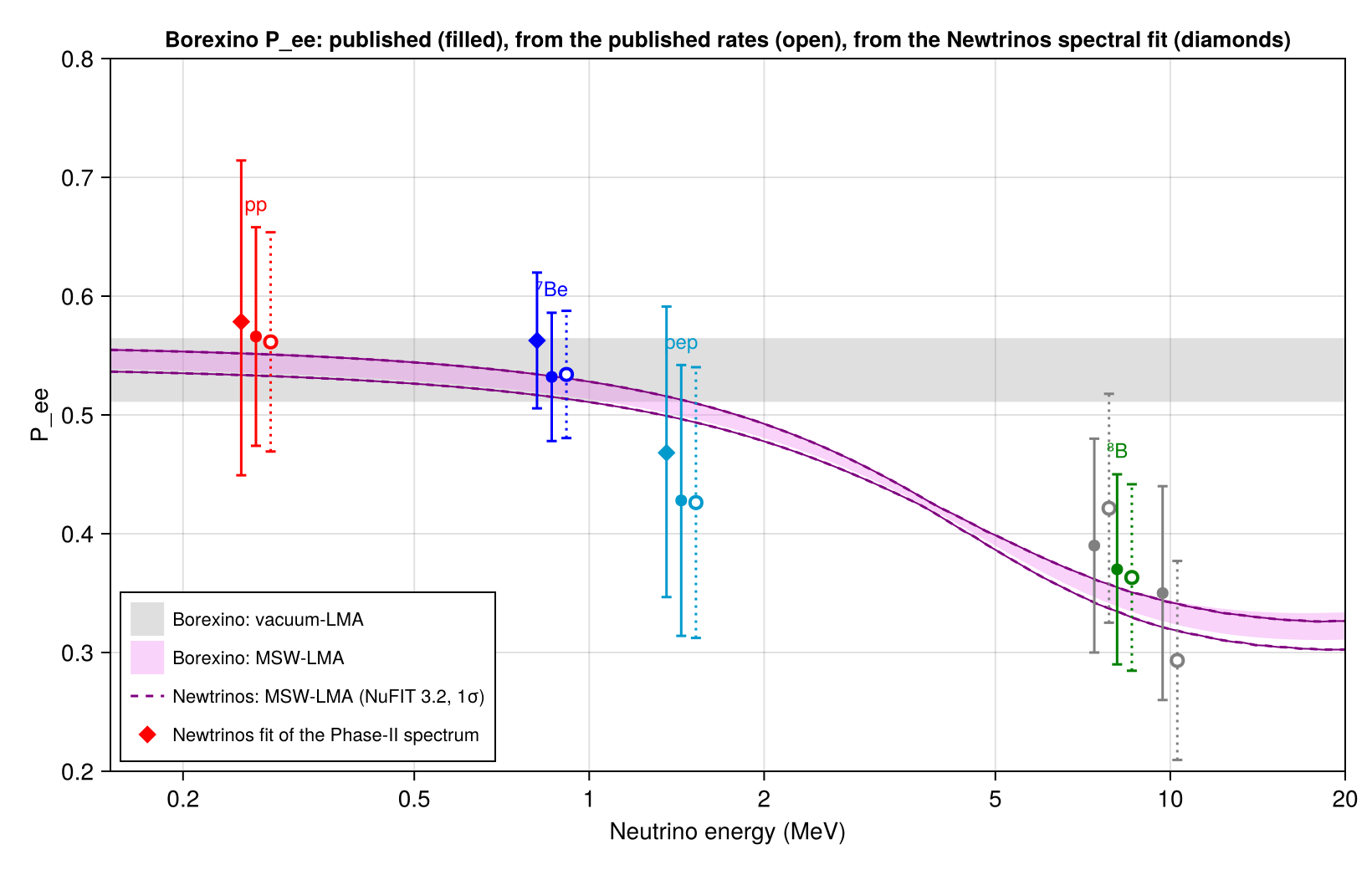
The electron-neutrino survival probability from the Borexino pp, ⁷Be, pep (Phase II, PRD 100, 082004) and ⁸B (PRD 101, 062001) interaction rates, compared with the MSW-LMA prediction (Fig. 3). Newtrinos inverts the published rates, R = N_e Φ [P ⟨σ_e⟩ + (1 − P) ⟨σ_x⟩], with its ν–e cross sections (solar_xsec) and the B16 high-metallicity fluxes used by Borexino, and finds P_ee = 0.561 ± 0.092 (pp), 0.534 ± 0.054 (⁷Be), 0.426 ± 0.114 (pep) and 0.363 ± 0.078 (⁸B, T > 3.2 MeV), against Borexino's 0.566 ± 0.092, 0.532 ± 0.054, 0.428 ± 0.114 and 0.37 ± 0.08. The Newtrinos MSW-LMA prediction (adiabatic conversion averaged over the ⁸B production region, Earth regeneration at LNGS, yearly average) agrees with the centre of Borexino's band within 0.008. With the NuFIT 3.2 best fit and the B23 MB22-met fluxes, the borexino_ph2 module predicts 130.9 (pp), 47.6 (⁷Be) and 2.72 (pep) cpd/100 t, against the B16-HZ predictions 131.1, 47.9 and 2.74 quoted by Borexino. Newtrinos' own fit of the Phase-II TFC-subtracted spectrum (module borexino_ph2_spectrum, open data of Fig. 2a; pp, ⁷Be, pep free, CNO at the HZ prediction, see the PRD 100, 082004 entry) gives pp = 136 [118, 155], ⁷Be = 50.0 [48.5, 51.5] and pep = 2.58 [2.15, 3.02] cpd/100 t, i.e. P_ee = 0.578 −0.129/+0.136 (pp), 0.563 ± 0.057 (⁷Be) and 0.468 −0.121/+0.123 (pep), consistent with Borexino's values (diamonds in the figure).
Figures
Electron-neutrino survival probability vs. neutrino energy: published, from the published rates, and from the Newtrinos spectral fit · Fig. 3
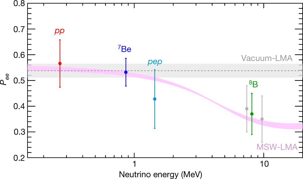
Original figure: Borexino, Nature 562, 505–510 (2018), Fig. 3, doi:10.1038/s41586-018-0624-y. Not our work; shown for comparison, all rights with the authors and publisher.
Known limitations
- Open points: inversion of the published Phase-II rates (the
borexino_ph2module uses these rates with the correlations as emulated by Super-Kamiokande). Diamonds: rates from the Newtrinos spectral fit (borexino_ph2_spectrum), which uses only the public TFC-subtracted energy spectrum (no radial or pulse-shape information, no TFC-tagged spectrum), so its pp interval is wider; its closure test on Borexino's best-fit model returns a pp rate 9 % low (see the PRD 100, 082004 entry). The spectral-fit errors are the profile-likelihood 68 % intervals of the rates combined with the B16-HZ flux uncertainty. - The Nature article text is not openly available; Borexino's points and bands are taken from the Borexino open data (Nature2018_Fig3_DATApoints/bands), the rates and the B16 predictions from the companion paper PRD 100, 082004 (arXiv:1707.09279), the ⁸B rates from PRD 101, 062001 (arXiv:1709.00756).
- The Newtrinos band is the envelope of the 1σ corners of sin²θ₁₂ and Δm²₂₁ of NuFIT 3.2 (sin²θ₁₃ = 0.02206), computed for the ⁸B production region at all energies; Borexino's prescription may differ (its band is narrower above 10 MeV). The small wiggles above 10 MeV come from the 20 night bins in cos(zenith) of the module's site.
- ⁸B sub-ranges: the inversion uses sharp recoil-energy thresholds (3.2 and 5.7 MeV), no energy resolution or efficiency, and a P_ee constant over the window. For the full HER range this reproduces Borexino (0.363 vs 0.37), for HER-I and HER-II it gives 0.421 and 0.293 against 0.39 and 0.35 (well within the errors).
- Errors: rate errors symmetrised (stat ⊕ syst) plus the B16-HZ flux uncertainty; with the B23 MB22-met fluxes of Newtrinos instead, P_ee(pp, ⁷Be, pep) changes by less than 0.01 and P_ee(⁸B) increases by about 0.03–0.04 (B23 ⁸B flux 6 % lower).
Reproduce
git clone https://github.com/Newtrinos-org/Newtrinos.jl.git && cd Newtrinos.jl && git checkout c6612c255a- Download reproduce.jl and the
data/folder of this entry into an empty directory. julia -t 8 --project=/path/to/Newtrinos.jl reproduce.jl
# Reproduction of Borexino, "Comprehensive measurement of pp-chain solar neutrinos", Nature 562, 505 (2018), Fig. 3:
# the electron-neutrino survival probability P_ee(E) from the pp, ⁷Be, pep and ⁸B interaction rates, compared with the
# MSW-LMA prediction. Borexino's points and bands are from the Borexino open data (data/Nature2018_Fig3_*.txt).
# Run from this directory with the Newtrinos.jl environment at the pinned commit:
#   julia -t 16 --project=<path to Newtrinos.jl> reproduce.jl
using Newtrinos, CairoMakie, CSV, DataFrames, DelimitedFiles, Printf
using Distributions, DensityInterface, Optim, ADTypes, ForwardDiff

cd(@__DIR__); mkpath("ours"); mkpath("results")
const SC = Newtrinos.solar_common
const NE = 3.307e31          # target electrons per 100 t
const DAY = 86400.0

bx = Newtrinos.borexino_ph2.configure()
physics, site = bx.physics, bx.assets.site          # LNGS, 42.45° N
sf = physics.solar_flux
p0 = Newtrinos.get_params((borexino_ph2 = bx,))
# oscillation parameters: NuFIT 3.2 (2018) best fit and 1σ ranges of sin²θ₁₂ and Δm²₂₁
osc(s12, dm) = merge(p0, (θ₁₂ = asin(sqrt(s12)), θ₁₃ = asin(sqrt(0.02206)), Δm²₂₁ = dm))
s12_bf, s12_lo, s12_hi = 0.307, 0.295, 0.320
dm_bf, dm_lo, dm_hi = 7.40e-5, 7.20e-5, 7.61e-5
pbf = osc(s12_bf, dm_bf)

# --- MSW-LMA band: yearly (day + night) averaged P_ee at LNGS, ⁸B production region, envelope of the 1σ corners ---
E = exp.(range(log(0.1), log(20.0), length = 120))
Pee(p) = SC.averaged_prob(physics, site, :b8, E, p)[:, 1]
curves = [Pee(osc(s, d)) for s in (s12_lo, s12_bf, s12_hi), d in (dm_lo, dm_bf, dm_hi)]
P_mid = Pee(pbf); P_min = minimum(reduce(hcat, vec(curves)), dims = 2)[:]; P_max = maximum(reduce(hcat, vec(curves)), dims = 2)[:]
bands = readdlm("data/Nature2018_Fig3_DATAbands.txt", skipstart = 2)
Eb, lmin, lmax, vmin, vmax = bands[:, 2], bands[:, 3], bands[:, 4], bands[:, 5], bands[:, 6]
bx_mid(e) = (i = clamp(searchsortedfirst(Eb, e), 2, length(Eb)); (lmin[i] + lmax[i]) / 2)
dev = maximum(abs.(P_mid .- bx_mid.(E)))
@printf("Newtrinos LMA P_ee (NuFIT 3.2 best fit) vs centre of Borexino's MSW-LMA band: max |Δ| = %.3f over 0.1–20 MeV\n", dev)

# --- "measured" P_ee from the published rates: R = N_e Φ [P ⟨σ_e⟩ + (1 − P) ⟨σ_x⟩] ---
# flux-averaged ν–e cross sections [cm²] above the recoil threshold T_min (continuum: Newtrinos spectral shape)
function σavg(comp; T_min = 0.0, T_max = Inf)
    est = SC.ESTotal(physics, comp; T_min)
    w = est.line ? est.w : est.w .* sf.spectrum(comp, est.E, p0) ./ sf.flux(comp, p0)   # normalised to the total flux
    σe, σx = sum(w .* est.σe), sum(w .* est.σx)
    isfinite(T_max) || return σe, σx
    he, hx = σavg(comp; T_min = T_max)                  # recoil window [T_min, T_max]
    σe - he, σx - hx
end
# total fluxes [cm⁻² s⁻¹]: B16 (GS98) high-metallicity SSM as used by Borexino, and Newtrinos' B23 MB22-met
Φ_HZ = (pp = 5.98e10, be7 = 4.93e9, pep = 1.44e8, b8 = 5.46e6)
Φ_HZ_unc = (pp = 0.006, be7 = 0.06, pep = 0.009, b8 = 0.12)
# measurements [cpd/100 t]: Phase II (PRD 100, 082004; pep with CNO at the HZ prediction) and ⁸B (PRD 101, 062001)
meas = [
    (name = "pp", comp = :pp, E = 0.267, R = 134.0, up = hypot(10, 6), dn = hypot(10, 10), kw = (;)),
    (name = "⁷Be", comp = :be7, E = 0.862, R = 48.3, up = hypot(1.1, 0.4), dn = hypot(1.1, 0.7), kw = (;)),
    (name = "pep", comp = :pep, E = 1.44, R = 2.43, up = hypot(0.36, 0.15), dn = hypot(0.36, 0.22), kw = (;)),
    (name = "⁸B HER-I", comp = :b8, E = 7.4, R = 0.136, up = hypot(0.013, 0.003), dn = hypot(0.013, 0.003), kw = (T_min = 3.2, T_max = 5.7)),
    (name = "⁸B HER", comp = :b8, E = 8.1, R = 0.223, up = hypot(0.015, 0.006), dn = hypot(0.016, 0.006), kw = (T_min = 3.2,)),
    (name = "⁸B HER-II", comp = :b8, E = 9.7, R = 0.087, up = hypot(0.010, 0.005), dn = hypot(0.010, 0.005), kw = (T_min = 5.7,)),
]
pts = readdlm("data/Nature2018_Fig3_DATApoints.txt")
bx_pts = Dict{Float64, Tuple{Float64, Float64}}()
for i in axes(pts, 1)
    pts[i, 1] isa Number && pts[i, 2] isa Number && (bx_pts[pts[i, 1]] = (pts[i, 2], pts[i, 3]))
end
rows = []
for m in meas
    σe, σx = σavg(m.comp; m.kw...)
    Pfrom(R, Φ) = (R / (NE * DAY * Φ) - σx) / (σe - σx)
    Φh = Φ_HZ[m.comp]; Φb = sf.flux(m.comp, p0)
    P_HZ = Pfrom(m.R, Φh)
    err = sqrt(((m.up + m.dn) / 2 / (NE * DAY * Φh * (σe - σx)))^2 + (Φ_HZ_unc[m.comp] * (P_HZ + σx / (σe - σx)))^2)
    # predicted rate at the NuFIT 3.2 best fit with Newtrinos' fluxes, P_ee averaged over the spectrum
    est = SC.ESTotal(physics, m.comp; T_min = get(m.kw, :T_min, 0.0))
    R_pred = SC.es_interaction_rate(physics, site, est, pbf) * NE * DAY
    if haskey(m.kw, :T_max)
        R_pred -= SC.es_interaction_rate(physics, site, SC.ESTotal(physics, m.comp; T_min = m.kw.T_max), pbf) * NE * DAY
    end
    push!(rows, (measurement = m.name, E_MeV = m.E, rate_cpd100t = m.R, rate_newtrinos_cpd100t = R_pred,
                 Pee_borexino = bx_pts[m.E][1], Pee_borexino_err = bx_pts[m.E][2],
                 Pee_newtrinos_B16HZ = P_HZ, Pee_newtrinos_B16HZ_err = err, Pee_newtrinos_B23 = Pfrom(m.R, Φb),
                 sigma_e_cm2 = σe, sigma_x_cm2 = σx))
end
df = DataFrame(rows)
CSV.write("results/pee_rates.csv", df)
show(stdout, df[:, 1:9]; allrows = true); println()

# --- P_ee from Newtrinos' own fit of the Phase-II TFC-subtracted spectrum (borexino_ph2_spectrum, open data of Fig. 2a):
#     pp, ⁷Be, pep free, CNO constrained to the HZ prediction 4.92 ± 0.56 cpd/100 t, as in PRD 100, 082004 ---
const BS = Newtrinos.borexino_ph2_spectrum
sphys = merge(BS.default_physics(), (solar_flux = Newtrinos.solar_flux.configure(
    Newtrinos.solar_flux.SolarFluxConfig(systematics = Newtrinos.solar_flux.SSMPriors())),))
bs = BS.configure(sphys)
sllh = Newtrinos.generate_likelihood((borexino_ph2_spectrum = bs,))
sp0 = Newtrinos.get_params((borexino_ph2_spectrum = bs,)); spri = Newtrinos.get_priors((borexino_ph2_spectrum = bs,))
rate0 = BS.solar_rates(sp0, bs.physics, bs.assets)
nuis = collect(keys(bs.params))
toparams(x) = merge(sp0, (solar_norm_pp = x[1], solar_norm_be7 = x[2], solar_norm_pep = x[3],
                          solar_norm_n13 = x[4], solar_norm_o15 = x[4], solar_norm_f17 = x[4]),
                    NamedTuple{Tuple(nuis)}(Tuple(x[5:end])))
cno_prior = Normal(4.92, 0.56)
nlp(x) = -(logdensityof(sllh, toparams(x)) + logpdf(cno_prior, x[4] * rate0.cno) +
           sum(logpdf(spri[k], x[4+i]) for (i, k) in enumerate(nuis)))
lo = vcat(0.2, 0.5, 0.0, 0.0, [minimum(spri[k]) for k in nuis]); hi = vcat(2.0, 1.5, 3.0, 3.0, [maximum(spri[k]) for k in nuis])
function minimise(f, x0, lo, hi)
    r = optimize(f, lo, hi, clamp.(x0, lo .+ 1e-6, hi .- 1e-6), Fminbox(LBFGS()),
                 Optim.Options(iterations = 1000, outer_iterations = 10, g_tol = 1e-6); autodiff = ADTypes.AutoForwardDiff())
    Optim.minimizer(r), Optim.minimum(r)
end
xb, mb = minimise(nlp, vcat(1.0, 1.0, 1.0, 4.92 / rate0.cno, [sp0[k] for k in nuis]), lo, hi)
sbest = BS.solar_rates(toparams(xb), bs.physics, bs.assets)
# 68 % intervals of each rate from its profile (−2Δln L = 1), scanned outwards from the best fit
grids = (pp = collect(90.0:5.0:180.0), be7 = collect(44.0:0.5:53.0), pep = collect(1.0:0.2:4.0))
sint = Dict{Symbol, Tuple{Float64, Float64}}()
lk = ReentrantLock()
Threads.@threads for (i, k) in collect(enumerate((:pp, :be7, :pep)))
    g = grids[k]; prof = zeros(length(g)); keep = setdiff(eachindex(xb), i)
    ib = searchsortedfirst(g, sbest[k])
    for order in (ib:length(g), reverse(1:ib-1))
        ystart = xb[keep]
        for j in order
            fix(y) = (x = Vector{eltype(y)}(undef, length(xb)); x[keep] = y; x[i] = g[j] / rate0[k]; x)
            r1 = minimise(y -> nlp(fix(y)), ystart, lo[keep], hi[keep])
            r2 = minimise(y -> nlp(fix(y)), xb[keep], lo[keep], hi[keep])
            y, m = r1[2] <= r2[2] ? r1 : r2
            prof[j] = 2 * (m - mb); ystart = y
        end
    end
    gg = vcat(g, sbest[k]); pp_ = vcat(prof, 0.0); o = sortperm(gg); gg, pp_ = gg[o], pp_[o]
    jb = findfirst(==(0.0), pp_)
    cross(i1, i2) = gg[i1] + (1 - pp_[i1]) * (gg[i2] - gg[i1]) / (pp_[i2] - pp_[i1])
    il = findlast(>(1), pp_[1:jb]); iu = jb - 1 + findfirst(>(1), pp_[jb:end])
    lock(lk) do
        sint[k] = ((il === nothing ? NaN : cross(il, il + 1)), (iu === nothing ? NaN : cross(iu - 1, iu)))
    end
end
srows = map(((:pp, "pp"), (:be7, "⁷Be"), (:pep, "pep"))) do (k, name)
    m = meas[findfirst(x -> x.name == name, meas)]
    σe, σx = σavg(m.comp)
    Pfrom(R) = (R / (NE * DAY * Φ_HZ[m.comp]) - σx) / (σe - σx)
    Pl, Pu = Pfrom(sint[k][1]), Pfrom(sint[k][2])
    P = Pfrom(sbest[k])
    # rate interval ⊕ B16-HZ flux uncertainty
    flux = Φ_HZ_unc[m.comp] * (P + σx / (σe - σx))
    (measurement = name, E_MeV = m.E, rate_cpd100t = sbest[k], rate_lo = sint[k][1], rate_hi = sint[k][2],
     Pee = P, Pee_err_lo = hypot(P - Pl, flux), Pee_err_hi = hypot(Pu - P, flux))
end
sdf = DataFrame(collect(srows))
CSV.write("results/pee_spectral_fit.csv", sdf)
show(stdout, sdf; allrows = true); println()

# predicted vs measured rates with the B16 SSM predictions of PRD 100, 082004 (Table V)
open("results/summary.txt", "w") do io
    println(io, "Interaction rates [cpd/100 t]: measured | Newtrinos (B23 MB22-met, NuFIT 3.2) | B16-HZ | B16-LZ (PRD 100, 082004, Table V)")
    ssm = Dict("pp" => (131.1, 132.2), "⁷Be" => (47.9, 43.7), "pep" => (2.74, 2.78))
    for r in eachrow(df)
        h = get(ssm, r.measurement, (NaN, NaN))
        @printf(io, "  %-10s %8.3f | %8.3f | %7.2f | %7.2f\n", r.measurement, r.rate_cpd100t, r.rate_newtrinos_cpd100t, h...)
    end
    println(io, "P_ee: Borexino | Newtrinos from the rates with B16-HZ fluxes | with B23 MB22-met fluxes")
    for r in eachrow(df)
        @printf(io, "  %-10s %.3f ± %.3f | %.3f ± %.3f | %.3f\n", r.measurement, r.Pee_borexino, r.Pee_borexino_err,
                r.Pee_newtrinos_B16HZ, r.Pee_newtrinos_B16HZ_err, r.Pee_newtrinos_B23)
    end
    println(io, "P_ee from the Newtrinos fit of the Phase-II spectrum (borexino_ph2_spectrum, B16-HZ fluxes): rate [68 % CL] -> P_ee")
    for r in eachrow(sdf)
        @printf(io, "  %-10s %7.2f [%.2f, %.2f] -> %.3f −%.3f +%.3f\n", r.measurement, r.rate_cpd100t, r.rate_lo, r.rate_hi,
                r.Pee, r.Pee_err_lo, r.Pee_err_hi)
    end
    @printf(io, "LMA P_ee (NuFIT 3.2 best fit, ⁸B production, LNGS) vs centre of Borexino's band: max |Δ| = %.3f\n", dev)
end
print(read("results/summary.txt", String))

# --- figure in the style of Fig. 3 ---
fig = Figure(size = (820, 520))
ax = Axis(fig[1, 1], xscale = log10, xlabel = "Neutrino energy (MeV)", ylabel = "P_ee",
          title = "Borexino P_ee: published (filled), from the published rates (open), from the Newtrinos spectral fit (diamonds)", titlesize = 13,
          xticks = ([0.2, 0.5, 1, 2, 5, 10, 20], ["0.2", "0.5", "1", "2", "5", "10", "20"]))
sel = 0.15 .<= Eb .<= 20
band!(ax, Eb[sel], vmin[sel], vmax[sel], color = (:gray, 0.25), label = "Borexino: vacuum-LMA")
band!(ax, Eb[sel], lmin[sel], lmax[sel], color = (:violet, 0.35), label = "Borexino: MSW-LMA")
band!(ax, E, P_min, P_max, color = (:purple, 0.0), strokecolor = :purple, strokewidth = 1)
lines!(ax, E, P_min, color = :purple, linestyle = :dash, label = "Newtrinos: MSW-LMA (NuFIT 3.2, 1σ)")
lines!(ax, E, P_max, color = :purple, linestyle = :dash)
colors = [:red, :blue, :deepskyblue3, :gray, :green, :gray]
for (i, r) in enumerate(eachrow(df))
    errorbars!(ax, [r.E_MeV], [r.Pee_borexino], [r.Pee_borexino_err], color = colors[i], whiskerwidth = 6)
    scatter!(ax, [r.E_MeV], [r.Pee_borexino], color = colors[i], markersize = 10)
    x = r.E_MeV * 1.06
    errorbars!(ax, [x], [r.Pee_newtrinos_B16HZ], [r.Pee_newtrinos_B16HZ_err], color = colors[i], whiskerwidth = 6, linestyle = :dot)
    scatter!(ax, [x], [r.Pee_newtrinos_B16HZ], color = :white, strokecolor = colors[i], strokewidth = 2, markersize = 10)
    text!(ax, r.E_MeV, r.Pee_borexino + r.Pee_borexino_err + 0.01, text = split(r.measurement)[1] * (occursin("HER", r.measurement) ? "" : ""),
          align = (:center, :bottom), fontsize = 12, color = colors[i], visible = !occursin("HER-", r.measurement))
end
for (i, r) in enumerate(eachrow(sdf))
    x = r.E_MeV / 1.06
    rangebars!(ax, [x], [r.Pee - r.Pee_err_lo], [r.Pee + r.Pee_err_hi], color = colors[i], whiskerwidth = 6)
    scatter!(ax, [x], [r.Pee], color = colors[i], marker = :diamond, markersize = 12,
             label = i == 1 ? "Newtrinos fit of the Phase-II spectrum" : nothing)
end
xlims!(ax, 0.15, 20); ylims!(ax, 0.2, 0.8)
axislegend(ax, position = :lb, labelsize = 11)
save("ours/fig3_pee.png", fig)
Provenance
| Newtrinos.jl commit | c6612c255a (borexino_ph2_spectrum, borexino_ph2, solar_common, solar_flux, solar_xsec, osc, earth_layers) |
|---|---|
| Run date | 2026-10-21T16:52:17Z |
| Wall time | 5.2 min (128 threads) |
| Julia | 1.12.5 |
| Machine | AMD EPYC 7702P 64-Core Processor, 128 hardware threads, Linux |
| Environment | newtrinos_Manifest.toml · run.toml |
Downloads
CSV files hold one row per scan point: the scanned and profiled parameters
(sin2_theta23, dm2_32 in eV², dcp in rad, nuisance parameters), dchi2 = −2Δ log L
and the log-likelihood. JLD2 files contain the full NewtrinosResult objects.
| File | Size | SHA-256 |
|---|---|---|
| ours/fig3_pee.png | 161.2 kB | f1c4729bc0e8… |
| results/pee_rates.csv | 1.1 kB | 66d46f25eaaa… |
| results/pee_spectral_fit.csv | 447 B | b599bab2285c… |
| results/summary.txt | 1.2 kB | 2aa57dd84f8b… |