
NOvA, T2K · Nature 646, 818–824 (2025)
Joint neutrino oscillation analysis from the T2K and NOvA experiments
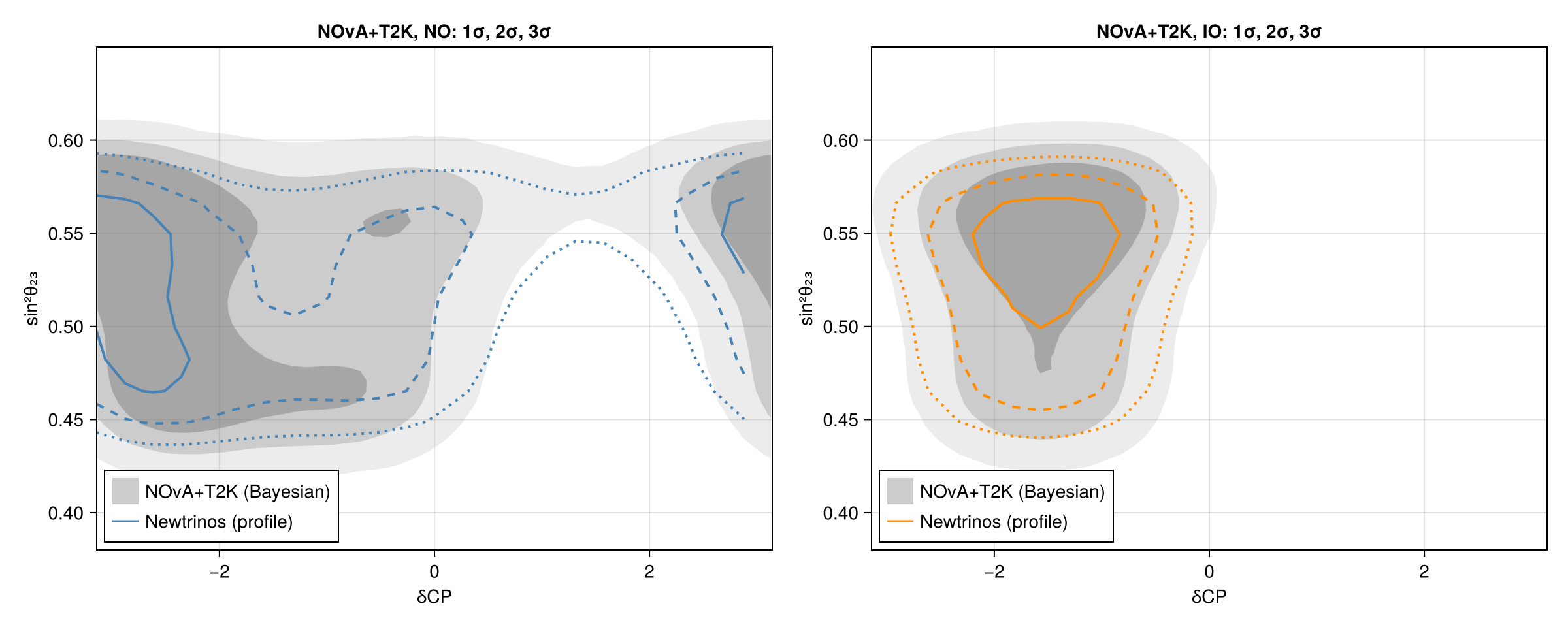
Joint fit of the Newtrinos NOvA and T2K modules as they are (no shared systematics), with the reactor constraint sin²θ₁₃ = 0.0218 ± 0.0007, compared with the official joint Bayesian analysis.
Figures
δCP – sin²θ₂₃, normal and inverted ordering · Fig. 3
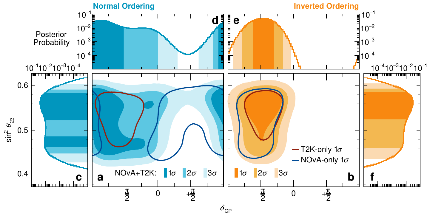
Original figure: NOvA, T2K, Nature 646, 818–824 (2025), Fig. 3, doi:10.1038/s41586-025-09599-3. Not our work; shown for comparison, all rights with the authors and publisher.
Known limitations
- Not like-for-like: the official analysis uses the NOvA 2020 data set and the T2K 2023 analysis; here NOvA 2024 (twice the ν exposure) and the T2K 2025 model are used.
- Newtrinos commit: feature/ordering-combo, i.e. main with the T2K fix (misidentified νμ CC background of the e-like samples oscillated with P_μμ), the NOvA fixes (per-bin νμ correction at the reference point, ντ CC background) and the ORCA fixes (unused here).
- Official results are Bayesian (marginalised, HPD); ours are profile likelihood.
- Best fits (results/bestfit_vs_official.toml): NO |Δm²₃₂| 2.450 (2.43), sin²θ₂₃ 0.548 (0.561), δCP −0.95π (−0.87π); IO 2.488 (2.48), 0.549 (0.563), −0.45π (−0.47π). Mass ordering: we prefer NO by Δχ² = 0.60, official Bayes factor 1.3 for IO.
Reproduce
git clone https://github.com/Newtrinos-org/Newtrinos.jl.git && cd Newtrinos.jl && git checkout c6612c255a- Download reproduce.jl and the
data/folder of this entry into an empty directory. julia -t 8 --project=/path/to/Newtrinos.jl reproduce.jl
# Reproduction of NOvA & T2K Collaborations, Nature 646, 818 (2025) [arXiv:2510.19888]: joint NOvA+T2K
# fit with the Newtrinos.jl modules `nova` (2024 data) and `t2k` (2025 analysis) as they are.
# Run from this directory with the Newtrinos.jl environment at the pinned commit:
#   julia -t 8 --project=<path to Newtrinos.jl> reproduce.jl
using Newtrinos, Distributions, DataStructures, Accessors, FileIO, CairoMakie, HDF5, CSV, DataFrames, Printf

cd(@__DIR__); mkpath("ours"); mkpath("results"); mkpath("cache")

# CSV export of a profile scan: one row per grid point, ASCII column names, oscillation parameters in physical
# units (sin²θ, Δm²₃₂ = Δm²₃₁ − Δm²₂₁ in eV², δCP in rad), dchi2 = -2Δlog L w.r.t. `ref` (default: the scan's best fit)
function save_csv(path, r; ref = maximum(r.values.log_posterior))
    ascii(k) = replace(string(k), "θ" => "theta", "Δm²" => "dm2_", "δ" => "d", "₁" => "1", "₂" => "2", "₃" => "3", "CP" => "cp")
    cols = OrderedDict{String,Any}()
    for (k, v) in pairs(r.values)
        x = vec(v)
        if startswith(string(k), "θ")
            cols["sin2_" * ascii(k)] = sin.(x) .^ 2
        elseif k == :Δm²₃₁
            cols["dm2_32"] = x .- vec(r.values.Δm²₂₁)
        end
        cols[ascii(k)] = x
    end
    cols["dchi2"] = 2 .* (ref .- vec(r.values.log_posterior))
    haskey(cols, "llh") && (cols["log_likelihood"] = pop!(cols, "llh"))
    first_cols = filter(in(keys(cols)), ["sin2_theta23", "dm2_32", "dcp", "dchi2", "log_likelihood", "log_posterior"])
    CSV.write(path, DataFrame(cols)[:, vcat(first_cols, setdiff(collect(keys(cols)), first_cols))])
end

# draw each confidence level with its own line style (1σ solid, 2σ dashed, 3σ dotted)
function contours!(ax, res, levels; color, label)
    for (lv, ls) in zip(levels, (:solid, :dash, :dot))
        plot!(ax, res, levels = [lv], color = color, linestyle = ls, label = lv == first(levels) ? label : nothing)
    end
end

experiments = (nova = Newtrinos.nova.configure(), t2k = Newtrinos.t2k.configure())
likelihood = Newtrinos.generate_likelihood(experiments)

# as in the paper: sin²θ₁₂ = 0.307 and Δm²₂₁ = 7.53e-5 eV² fixed, sin²θ₁₃ = 0.0218 ± 0.0007, flat δCP
θ₁₃ = asin(sqrt(0.0218))
θ₂₃_range = (asin(sqrt(0.35)), asin(sqrt(0.68)))
p = merge(Newtrinos.get_params(experiments), (θ₁₂ = asin(sqrt(0.307)), Δm²₂₁ = 7.53e-5, θ₁₃ = θ₁₃))
priors = merge(Newtrinos.get_priors(experiments),
               (θ₁₂ = p.θ₁₂, Δm²₂₁ = p.Δm²₂₁, θ₁₃ = Normal(θ₁₃, 0.0007 / (2 * sin(θ₁₃) * cos(θ₁₃))), δCP = Uniform(0, 2π), θ₂₃ = Uniform(θ₂₃_range...)))

orderings = (NO = (Δm²₃₂ = (2.25e-3, 2.65e-3), start = (Δm²₃₂ = 2.43e-3, δCP = mod(-0.87π, 2π)), color = :steelblue),
             IO = (Δm²₃₂ = (-2.65e-3, -2.25e-3), start = (Δm²₃₂ = -2.48e-3, δCP = mod(-0.47π, 2π)), color = :darkorange))

function profile_octants(pr, p0, vars, cache_dir)
    oct = map((lower = (θ₂₃_range[1], π / 4), upper = (π / 4, θ₂₃_range[2]))) do r
        Newtrinos.profile(likelihood, @set(pr.θ₂₃ = Uniform(r...)), vars, @set(p0.θ₂₃ = sum(r) / 2), cache_dir = cache_dir)
    end
    # the two octant scans use θ₂₃ priors of different widths, which shifts each log_posterior by its own
    # constant −log(width): remove it before comparing the octants (nuisance-parameter priors are kept)
    widths = (lower = π / 4 - θ₂₃_range[1], upper = θ₂₃_range[2] - π / 4)
    oct = map((r, w) -> Newtrinos.NewtrinosResult(axes = r.axes, meta = r.meta,
                                                   values = merge(r.values, (log_posterior = r.values.log_posterior .+ log(w),))), oct, widths)
    better = oct.lower.values.log_posterior .>= oct.upper.values.log_posterior
    Newtrinos.NewtrinosResult(axes = oct.lower.axes, values = map((l, u) -> ifelse.(better, l, u), oct.lower.values, oct.upper.values), meta = oct.lower.meta)
end

results = map(keys(orderings), values(orderings)) do mo, o
    pr = @set priors.Δm²₃₁ = Uniform((o.Δm²₃₂ .+ p.Δm²₂₁)...)
    p0 = merge(p, (Δm²₃₁ = o.start.Δm²₃₂ + p.Δm²₂₁, δCP = o.start.δCP, θ₂₃ = asin(sqrt(0.56))))
    dcp = profile_octants(pr, p0, OrderedDict(:δCP => 41), "cache/$(mo)_dcp")
    dcpth23 = Newtrinos.profile(likelihood, pr, OrderedDict(:δCP => 25, :θ₂₃ => 21), p0, cache_dir = "cache/$(mo)_dcpth23")
    FileIO.save("results/nova_t2k_$(mo).jld2", Dict("dcp" => dcp, "dcpth23" => dcpth23))
    mo => (; dcp, dcpth23)
end |> NamedTuple
# Δχ² references: each scan type carries the log density of its own scanned-parameter priors, so a scan is
# referenced to the best fit over both orderings of the same scan type
scan_max(k) = maximum(r -> maximum(r[k].values.log_posterior), results)
global_max = maximum(r -> maximum(r.dcp.values.log_posterior), results)
for mo in keys(results)   # dchi2 relative to the global best fit over both orderings
    save_csv("results/nova_t2k_$(mo)_dcp.csv", results[mo].dcp; ref = global_max)
    save_csv("results/nova_t2k_$(mo)_dcp_ssth23.csv", results[mo].dcpth23; ref = scan_max(:dcpth23))
end

# Fig. 3: δCP – sin²θ₂₃, 1σ / 2σ / 3σ, per ordering, with the official Bayesian regions (data/, extracted from the vector figure)
wrap(x) = mod(x + π, 2π) - π
regions = h5open("data/joint_fig3_regions.h5") do f
    Dict(mo => Dict(l => [(read(f["$mo/$l/$i/dcp"]), read(f["$mo/$l/$i/ssth23"])) for i in keys(f["$mo/$l"])] for l in keys(f[mo])) for mo in keys(f))
end
fig = Figure(size = (1200, 480))
for (i, mo) in enumerate(keys(orderings))
    ax = Axis(fig[1, i], title = "NOvA+T2K, $(mo): 1σ, 2σ, 3σ", xlabel = "δCP", ylabel = "sin²θ₂₃")
    for (lv, a) in (("3sigma", 0.15), ("2sigma", 0.3), ("1sigma", 0.5)), poly in get(regions[string(mo)], lv, [])
        poly!(ax, Point2f.(poly...), color = (:gray, a), strokewidth = 0)
    end
    poly!(ax, Point2f[(10, 10), (10.1, 10), (10, 10.1)], color = (:gray, 0.4), label = "NOvA+T2K (Bayesian)")
    r = results[mo].dcpth23; d = wrap.(r.axes.δCP); k = sortperm(d)
    contours!(ax, Newtrinos.NewtrinosResult(axes = (dcp = d[k], ss23 = sin.(r.axes.θ₂₃) .^ 2), values = map(v -> v[k, :], r.values)), [0.6827, 0.9545, 0.9973]; color = orderings[mo].color, label = "Newtrinos (profile)")
    xlims!(ax, -π, π); ylims!(ax, 0.38, 0.65)
    axislegend(ax, position = :lb)
end
save("ours/fig3_dcp_ssth23.png", fig)

# best fits vs. Extended Data Table III (Bayesian highest-posterior values)
official = (NO = (dm2 = 2.43, ss23 = 0.561, dcp = -0.87), IO = (dm2 = 2.48, ss23 = 0.563, dcp = -0.47))
open("results/bestfit_vs_official.toml", "w") do io
    for mo in keys(orderings)
        r = results[mo].dcp; i = argmax(r.values.log_posterior)
        @printf(io, "[%s]\nabs_dm2_32 = %.4f  # official %.2f (1e-3 eV²)\nsin2_theta23 = %.4f  # official %.3f\ndcp_over_pi = %.3f  # official %.2f\nminus2_dlogL_vs_global = %.3f\n\n",
                mo, abs(r.values.Δm²₃₁[i] - p.Δm²₂₁) * 1e3, official[mo].dm2, sin(r.values.θ₂₃[i])^2, official[mo].ss23,
                wrap(r.axes.δCP[i]) / π, official[mo].dcp, 2 * (global_max - r.values.log_posterior[i]))
    end
end
Provenance
| Newtrinos.jl commit | c6612c255a (nova, t2k) |
|---|---|
| Run date | 2026-10-21T15:58:01Z |
| Wall time | 4.4 min (128 threads) |
| Julia | 1.12.5 |
| Machine | AMD EPYC 7702P 64-Core Processor, 128 hardware threads, Linux |
| Environment | newtrinos_Manifest.toml · run.toml |
Downloads
CSV files hold one row per scan point: the scanned and profiled parameters
(sin2_theta23, dm2_32 in eV², dcp in rad, nuisance parameters), dchi2 = −2Δ log L
and the log-likelihood. JLD2 files contain the full NewtrinosResult objects.
| File | Size | SHA-256 |
|---|---|---|
| ours/fig3_dcp_ssth23.png | 215.5 kB | 89fc8b2322d8… |
| results/bestfit_vs_official.toml | 330 B | 6e4f21b655f8… |
| results/nova_t2k_IO.jld2 | 182.5 kB | a5ed54c9146f… |
| results/nova_t2k_IO_dcp.csv | 26.9 kB | 4cdec0932f64… |
| results/nova_t2k_IO_dcp_ssth23.csv | 337.5 kB | fc2fdad26f81… |
| results/nova_t2k_NO.jld2 | 182.5 kB | 5a907a75b037… |
| results/nova_t2k_NO_dcp.csv | 26.8 kB | a9f79c58751a… |
| results/nova_t2k_NO_dcp_ssth23.csv | 336.4 kB | 3d39ae170ee1… |