
E. Kh. Akhmedov, M. A. Tórtola, J. W. F. Valle · JHEP 05 (2004) 057
A simple analytic three-flavour description of the day-night effect in the solar neutrino flux
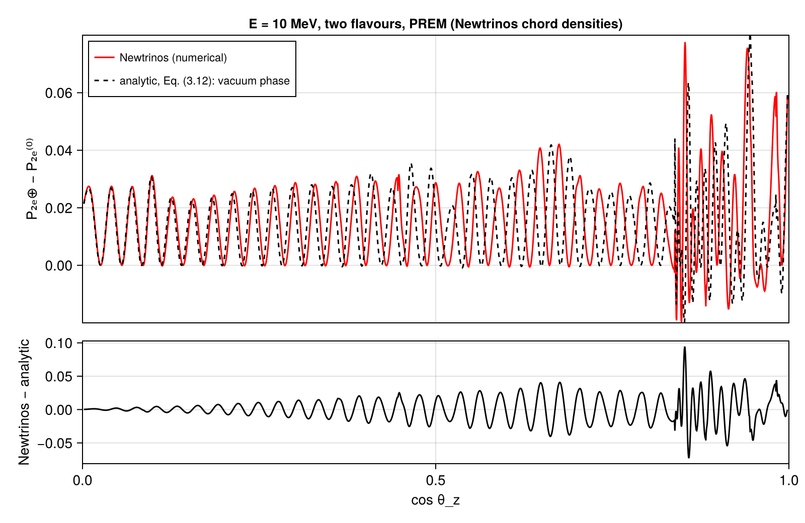
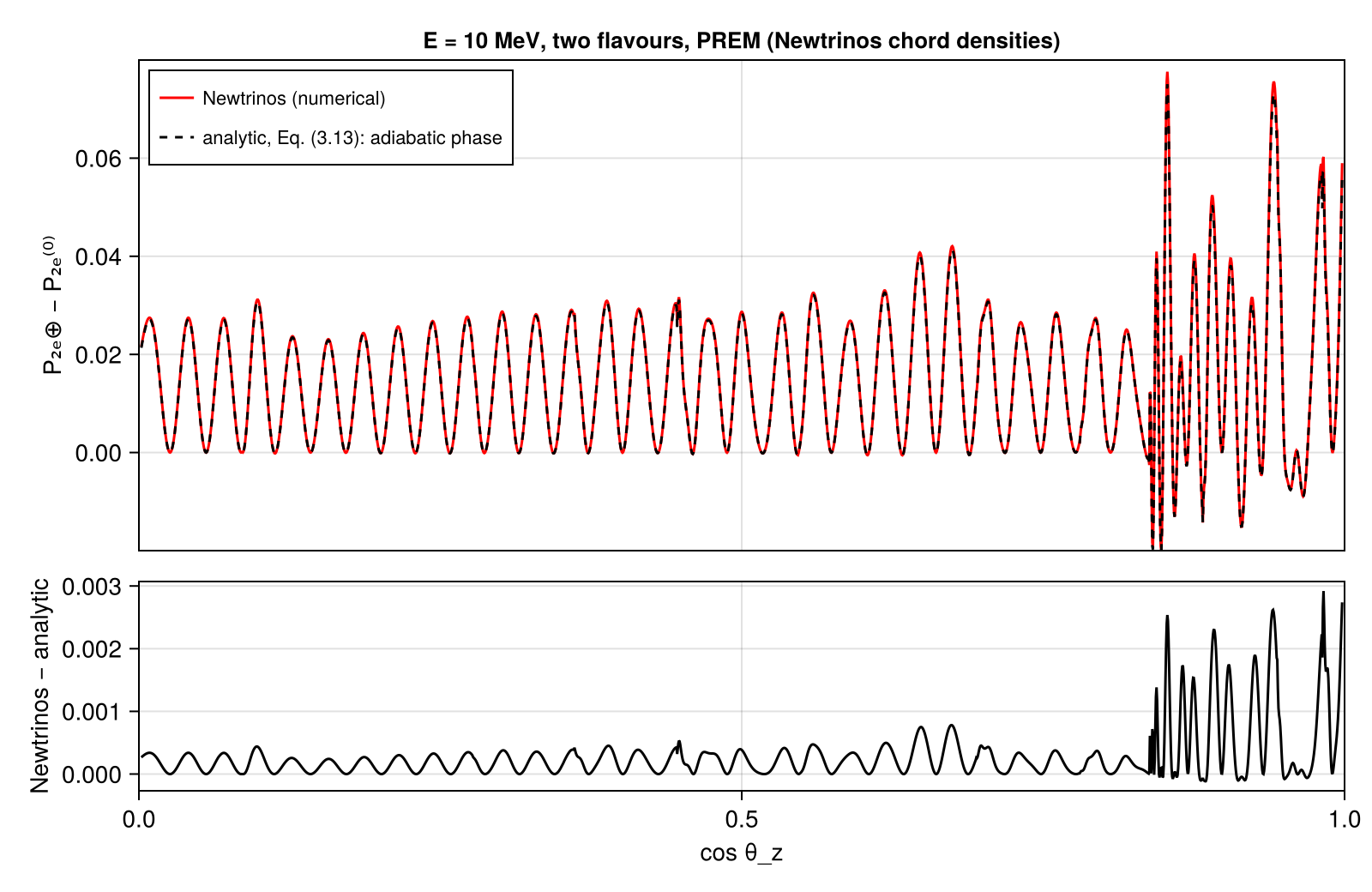
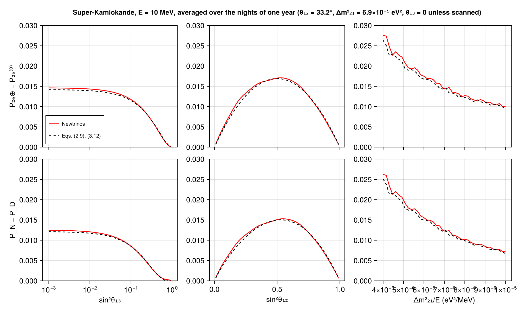
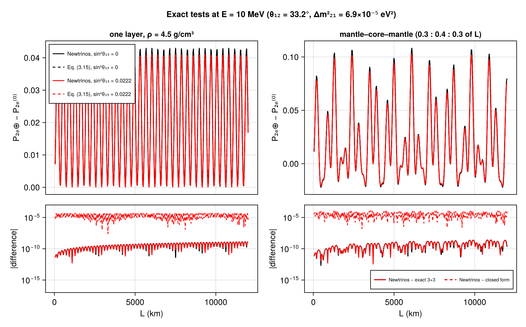
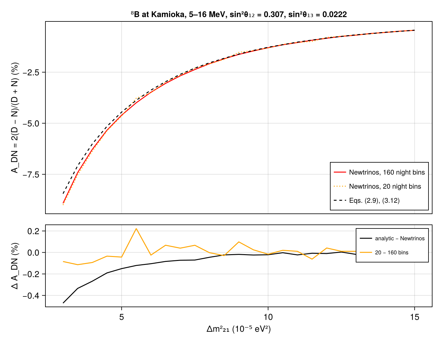
Earth regeneration of solar neutrinos in Newtrinos (mass eigenstates from the Sun propagated through layered Earth paths, osc.solar_prob) compared with the analytic three-flavour description of the paper: the regeneration factor f = P₂ₑ⊕ − P₂ₑ⁽⁰⁾ in the perturbative form of Eq. (3.12) and with the adiabatic phase, Eq. (3.13), the closed forms for one and three layers of constant density, Eqs. (3.15) and (3.19), and P_N − P_D = −c₁₃² cos2θ̂₁₂ f, Eq. (2.9). All formulas are evaluated on the density profile Newtrinos uses along each chord. Newtrinos agrees with an independent exact three-flavour propagation to 10⁻⁹ (one and three layers, any θ₁₃); along PREM chords at 10 MeV, Eq. (3.13) agrees to 5×10⁻⁴ rms, while Eq. (3.12) accumulates the phase error discussed in the paper (Figs. 1, 3). Averaged over one year at Super-Kamiokande (Fig. 4) the analytic and numerical f and P_N − P_D agree within 4×10⁻⁴–2.4×10⁻³, and the ⁸B day–night asymmetry agrees within 0.2–6 % of its value.
Figures
Regeneration factor vs. zenith angle at 10 MeV, Eq. (3.12) · Fig. 1
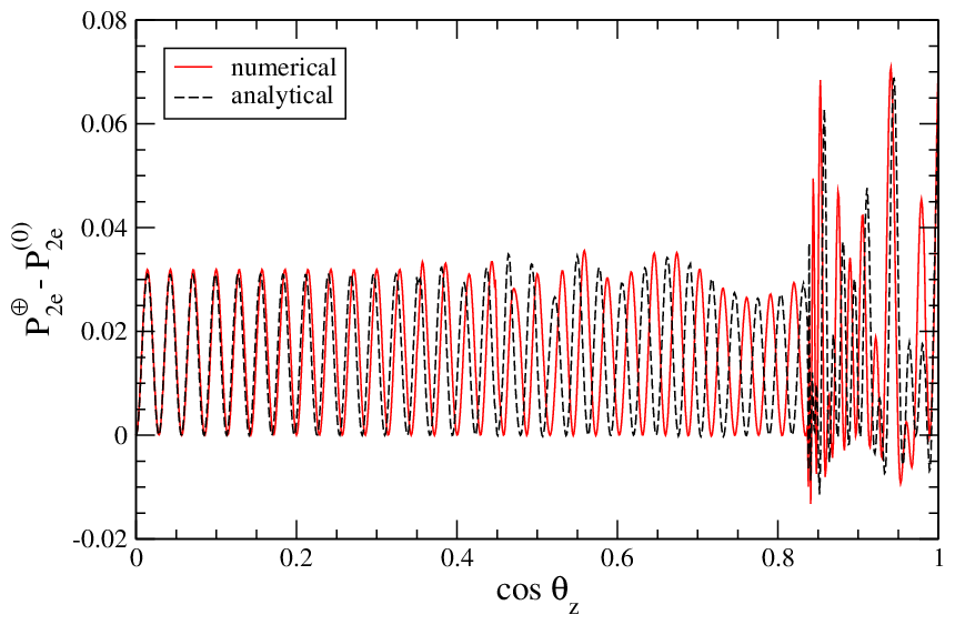
Original figure: E. Kh. Akhmedov, M. A. Tórtola, J. W. F. Valle, JHEP 05 (2004) 057, Fig. 1, doi:10.1088/1126-6708/2004/05/057. Not our work; shown for comparison, all rights with the authors and publisher.
Regeneration factor vs. zenith angle at 10 MeV, adiabatic phase, Eq. (3.13) · Fig. 3
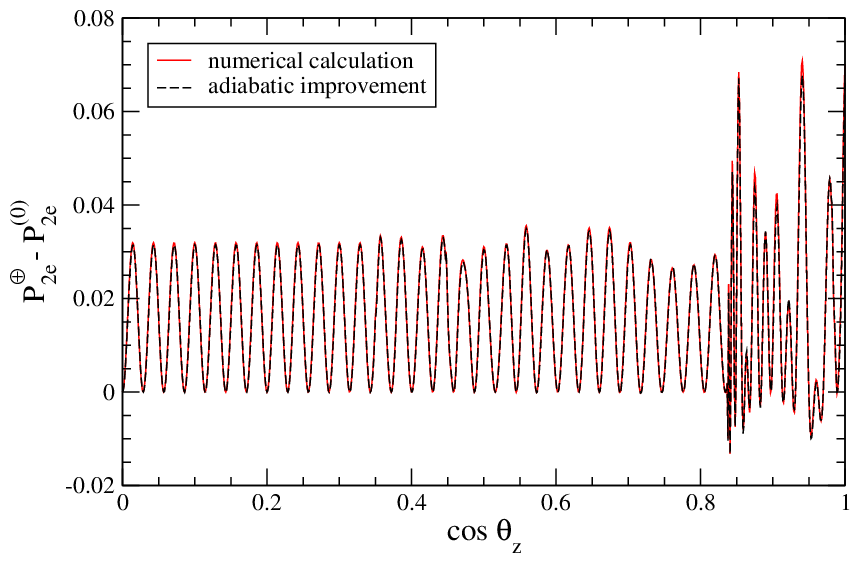
Original figure: E. Kh. Akhmedov, M. A. Tórtola, J. W. F. Valle, JHEP 05 (2004) 057, Fig. 3, doi:10.1088/1126-6708/2004/05/057. Not our work; shown for comparison, all rights with the authors and publisher.
Yearly averaged regeneration factor and P_N − P_D at Super-Kamiokande, 10 MeV · Fig. 4
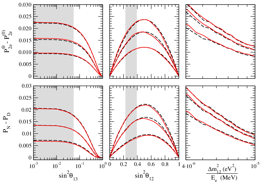
Original figure: E. Kh. Akhmedov, M. A. Tórtola, J. W. F. Valle, JHEP 05 (2004) 057, Fig. 4, doi:10.1088/1126-6708/2004/05/057. Not our work; shown for comparison, all rights with the authors and publisher.
Exact tests: one and three layers of constant density, Eqs. (3.15) and (3.19) · Eqs. (3.15), (3.19)
Eqs. (3.15), (3.19)
⁸B day–night asymmetry at Kamioka vs. Δm²₂₁ · Eqs. (2.9), (3.12)
Eqs. (2.9), (3.12)
Known limitations
- The paper's numerical curves come from an exact integration on PREM; here the analytic formulas are compared with Newtrinos on the Newtrinos Earth model for solar detectors (PREM zoned at its density discontinuities, with chord-averaged densities and continental crust instead of PREM's 3 km global ocean layer), so the original and reproduced figures differ in detail, e.g. in the regeneration amplitude for shallow paths.
- For θ₁₃ ≠ 0 the paper's two-flavour reduction (decoupled third state, potential c₁₃²V) differs from the exact three-flavour result by up to 5×10⁻⁵ (one layer) and 1.4×10⁻⁴ (three layers) at sin²θ₁₃ = 0.0222; Newtrinos follows the exact result.
- Fig. 4 is reproduced for the central parameters only (θ₁₂ = 33.2°, Δm²₂₁ = 6.9×10⁻⁵ eV², θ₁₃ = 0 unless scanned); the outer curves (3σ ranges of 2004) are not shown. The yearly averages use 160 night bins in cos θ_z at Kamioka (36.4° N, 1 km depth) and the ⁸B production region of B23.
- The ⁸B day–night asymmetry is weighted with the ⁸B spectrum × E between 5 and 16 MeV as a rough stand-in for the Super-K response. With 20 night bins (the default of the Newtrinos solar modules was 20; it is now 80) it differs from 160 bins by up to 0.23 % absolute (1–5 % relative).
- Fig. 2 (energy-averaged regeneration factor at Super-K) is not reproduced, since the paper does not specify the averaging.
Reproduce
git clone https://github.com/Newtrinos-org/Newtrinos.jl.git && cd Newtrinos.jl && git checkout c6612c255a- Download reproduce.jl into an empty directory.
julia -t 8 --project=/path/to/Newtrinos.jl reproduce.jl
# Verification of the Newtrinos.jl Earth regeneration of solar neutrinos (day/night effect, three flavours) against
# the analytic description of Akhmedov, Tórtola & Valle, JHEP 05 (2004) 057 [hep-ph/0404083].
# Newtrinos propagates the mass eigenstates arriving from the Sun through layered Earth paths (`osc.solar_prob`,
# `earth_mass_to_flavour`); here its regeneration factor f = P_2e^⊕ − |U_e2|² and P_N − P_D are compared with
#   - the exact two-flavour result for piecewise-constant density (independent 2×2 transfer matrices), which must agree
#     to machine precision for θ₁₃ = 0 (and up to O(s₁₃² V²/Δ²) for θ₁₃ ≠ 0 with the paper's c₁₃² V, c₁₃⁴ rules),
#   - the paper's perturbative formula, Eq. (3.12): f = c₁₃⁴ sin²2θ₁₂ ½ ∫₀ᴸ V(x) sin[2δ(L − x)] dx,
#   - its improved version with the adiabatic phase, Eq. (3.13),
#   - the closed forms for one and three layers of constant density, Eqs. (3.15) and (3.19),
#   - and P_N − P_D = −c₁₃² cos2θ̂₁₂ f, Eq. (2.9), with the production-averaged mixing angle in the Sun.
# All analytic formulas are evaluated on the same density profile along each chord that Newtrinos uses (PREM zones with
# chord-averaged densities), so the differences isolate implementation and approximation errors.
# Run from this directory with the Newtrinos.jl environment at the pinned commit:
#   julia -t 16 --project=<path to Newtrinos.jl> reproduce.jl
using Newtrinos, CairoMakie, CSV, DataFrames, LinearAlgebra, StructArrays, ArraysOfArrays, Printf

cd(@__DIR__); mkpath("ours"); mkpath("results")
const OSC = Newtrinos.osc
const HBARC = 1.973269804e-10          # eV·km
const V_PER_NE = OSC.A                  # √2 G_F N_A [eV per mol/cm³]

physics = Newtrinos.solar_common.default_physics()
osc, earth = physics.osc, physics.earth_layers
layers = earth.compute_layers()
prod_b8 = physics.solar_flux.production.b8

# parameters of the paper (best fit of Maltoni et al. 2003): θ₁₂ = 33.2°, Δm²₂₁ = 6.9e-5 eV², Δm²₃₁ = 2e-3 eV²
base = merge(Newtrinos.get_params((chlorine = Newtrinos.chlorine.configure(physics),)),
             (θ₁₂ = deg2rad(33.2), θ₁₃ = 0.0, θ₂₃ = π / 4, δCP = 0.0, Δm²₂₁ = 6.9e-5, Δm²₃₁ = 2e-3))
s13(p) = sin(p.θ₁₃); c13(p) = cos(p.θ₁₃)

# --- Newtrinos: P(ν_i → ν_e) through the Earth along `paths` -------------------------------------------------------
function newtrinos_P2e(E_MeV, paths, lay, p)
    U, h = OSC.get_matrices(osc.cfg.flavour, osc.cfg.eigen_method)(p)
    R = OSC.earth_mass_to_flavour(U, h .- minimum(h), E_MeV .* 1e-3, paths, lay, OSC.SI(), osc.cfg.eigen_method)
    R[:, :, 2, 1], abs2(U[1, 2])              # (n_E, n_paths), |U_e2|²
end
segments(path, lay) = [(seg.length, lay.p_density[seg.layer_idx]) for seg in path]   # (km, n_e [mol/cm³]), entry → detector

# --- analytic / independent two-flavour evolution in the (ν̃₁, ν̃₂) subspace (paper Eq. 2.11) ------------------------
δ_(E, p) = p.Δm²₂₁ / (4E * 1e6) / HBARC            # [1/km], E in MeV
V_(ne) = V_PER_NE * ne / HBARC                      # [1/km]
function exact_2f(E, segs, p)                        # exact for piecewise-constant density in the decoupling limit
    δ = δ_(E, p); s2, c2 = sin(2p.θ₁₂), cos(2p.θ₁₂)
    S = Matrix{ComplexF64}(I, 2, 2)
    for (ℓ, ne) in segs
        Vt = c13(p)^2 * V_(ne)
        H = [2sin(p.θ₁₂)^2 * δ + Vt  s2 * δ; s2 * δ  2cos(p.θ₁₂)^2 * δ]
        S = exp(-im * H * ℓ) * S
    end
    α, β = S[1, 1], S[1, 2]
    c13(p)^2 * (c2 * abs2(β) + s2 * real(conj(α) * β))     # Eq. (2.10)
end
# independent exact three-flavour propagation (PDG mixing matrix, flavour-basis Hamiltonian, matrix exponentials)
function exact_3f(E, segs, p)
    s12, c12, s13_, c13_, s23, c23 = sin(p.θ₁₂), cos(p.θ₁₂), sin(p.θ₁₃), cos(p.θ₁₃), sin(p.θ₂₃), cos(p.θ₂₃)
    eδ = cis(p.δCP)
    U = ComplexF64[c12*c13_ s12*c13_ s13_/eδ; -s12*c23-c12*s23*s13_*eδ c12*c23-s12*s23*s13_*eδ s23*c13_;
                   s12*s23-c12*c23*s13_*eδ -c12*s23-s12*c23*s13_*eδ c23*c13_]
    H0 = U * Diagonal([0.0, p.Δm²₂₁, p.Δm²₃₁]) * U' ./ (2E * 1e6) ./ HBARC       # [1/km]
    S = Matrix{ComplexF64}(I, 3, 3)
    for (ℓ, ne) in segs
        S = exp(-im * (H0 + Diagonal([V_(ne), 0.0, 0.0])) * ℓ) * S
    end
    abs2((S * U)[1, 2]) - abs2(U[1, 2])
end
function pert(E, segs, p; adiabatic = false)          # Eqs. (3.12) and (3.13)
    δ = δ_(E, p); s2, c2 = sin(2p.θ₁₂), cos(2p.θ₁₂)
    ω(ne) = sqrt((c2 * δ - c13(p)^2 * V_(ne) / 2)^2 + δ^2 * s2^2)
    L = sum(first, segs)
    # phase accumulated from the end of each segment to the detector
    k = adiabatic ? [ω(ne) for (_, ne) in segs] : fill(δ, length(segs))
    after = reverse(cumsum(reverse([ℓ * kk for ((ℓ, _), kk) in zip(segs, k)])))   # ∫ from start of segment to L
    acc = 0.0
    for (i, (ℓ, ne)) in enumerate(segs)
        rest = after[i] - ℓ * k[i]                      # ∫_{end of segment}^{L}
        # ∫_seg sin(2(rest + k(x_end − x))) dx = [1 − cos(2kℓ)]… evaluated exactly for constant k within the segment
        acc += V_(ne) * (cos(2rest) - cos(2(rest + k[i] * ℓ))) / (2k[i])
    end
    c13(p)^4 * s2^2 * acc / 2
end
function const_density(E, ne, L, p)                  # Eq. (3.15)
    δ = δ_(E, p); s2, c2 = sin(2p.θ₁₂), cos(2p.θ₁₂); V = V_(ne)
    ω = sqrt((c2 * δ - c13(p)^2 * V / 2)^2 + δ^2 * s2^2)
    c13(p)^4 * s2^2 * V * δ / (2ω^2) * sin(ω * L)^2
end
function three_layers(E, ne1, L1, ne2, L2, p)        # Eq. (3.19), mantle–core–mantle
    δ = δ_(E, p); s2, c2 = sin(2p.θ₁₂), cos(2p.θ₁₂)
    om(V) = sqrt((c2 * δ - c13(p)^2 * V / 2)^2 + δ^2 * s2^2)
    th(V) = 0.5 * atan(δ * s2, c2 * δ - c13(p)^2 * V / 2)
    V1, V2 = c13(p)^2 * V_(ne1), c13(p)^2 * V_(ne2)       # the formula is written for the potential c₁₃² V
    ω1, ω2 = om(V_(ne1)), om(V_(ne2)); t1, t2 = th(V_(ne1)), th(V_(ne2))
    Y = cos(ω1 * L1) * cos(ω2 * L2) - cos(2t1 - 2t2) * sin(ω1 * L1) * sin(ω2 * L2)
    c13(p)^2 * s2^2 * δ / (2ω1) * (2Y * sin(ω1 * L1) + ω1 / ω2 * sin(ω2 * L2)) *
        (V1 / ω1 * 2Y * sin(ω1 * L1) + V2 / ω2 * sin(ω2 * L2))
end
# production-averaged cos 2θ̂₁₂ in the Sun (Eqs. 2.3, 3.5 with c₁₃² V)
function cos2θ_sun(E, p)
    δ = δ_(E, p); s2, c2 = sin(2p.θ₁₂), cos(2p.θ₁₂); w = prod_b8.w ./ sum(prod_b8.w)
    sum(wk * (c2 * δ - c13(p)^2 * V_(ne) / 2) / sqrt((c2 * δ - c13(p)^2 * V_(ne) / 2)^2 + δ^2 * s2^2) for (wk, ne) in zip(w, prod_b8.ne))
end

# ===================================================================================================================
# 1. exact tests: one layer (mantle density) and three layers (mantle–core–mantle) of constant density
# ===================================================================================================================
mk_layers(nes) = StructArray{OSC.Layer}((fill(6371.0, length(nes)), collect(nes), collect(nes)))
ne_m, ne_c = 4.5 * 0.496, 11.5 * 0.467                 # mol/cm³
Ls = range(50, 12000, length = 400)
tests = DataFrame(L_km = Float64[], θ13 = Float64[], case = String[], newtrinos = Float64[], exact_3x3 = Float64[], exact_2x2 = Float64[],
                  closed_form = Float64[])
for θ13 in (0.0, asin(sqrt(0.0222)))
    p = merge(base, (θ₁₃ = θ13,))
    for L in Ls
        P, Ue2 = newtrinos_P2e([10.0], VectorOfVectors([[OSC.Path(L, 1)]]), mk_layers([ne_m]), p)
        push!(tests, (L, θ13, "1 layer", P[1] - Ue2, exact_3f(10.0, [(L, ne_m)], p), exact_2f(10.0, [(L, ne_m)], p),
                      const_density(10.0, ne_m, L, p)))
        L1, L2 = 0.3L, 0.4L
        P, Ue2 = newtrinos_P2e([10.0], VectorOfVectors([[OSC.Path(L1, 1), OSC.Path(L2, 2), OSC.Path(L1, 1)]]), mk_layers([ne_m, ne_c]), p)
        sg = [(L1, ne_m), (L2, ne_c), (L1, ne_m)]
        push!(tests, (L, θ13, "3 layers", P[1] - Ue2, exact_3f(10.0, sg, p), exact_2f(10.0, sg, p),
                      three_layers(10.0, ne_m, L1, ne_c, L2, p)))
    end
end
CSV.write("results/constant_density_tests.csv", tests)
for g in groupby(tests, [:θ13, :case])
    @printf("%-8s sin²θ₁₃ = %.4f: max |Newtrinos − exact 3×3| = %.1e, |Newtrinos − exact 2×2 (decoupled)| = %.1e, |Newtrinos − closed form| = %.1e (max f = %.3f)\n",
            g.case[1], sin(g.θ13[1])^2, maximum(abs.(g.newtrinos .- g.exact_3x3)), maximum(abs.(g.newtrinos .- g.exact_2x2)),
            maximum(abs.(g.newtrinos .- g.closed_form)), maximum(g.newtrinos))
end
fig = Figure(size = (900, 560))
for (j, case) in enumerate(("1 layer", "3 layers"))
    ax = Axis(fig[1, j], title = case == "1 layer" ? "one layer, ρ = 4.5 g/cm³" : "mantle–core–mantle (0.3 : 0.4 : 0.3 of L)",
              ylabel = "P₂ₑ⊕ − P₂ₑ⁽⁰⁾", titlesize = 13); hidexdecorations!(ax, grid = false)
    axr = Axis(fig[2, j], xlabel = "L (km)", ylabel = "|difference|", yscale = log10)
    for (θ13, c, lab) in ((0.0, :black, "sin²θ₁₃ = 0"), (asin(sqrt(0.0222)), :red, "sin²θ₁₃ = 0.0222"))
        g = tests[(tests.case .== case) .& (tests.θ13 .== θ13), :]
        lines!(ax, g.L_km, g.newtrinos, color = c, label = "Newtrinos, $lab")
        lines!(ax, g.L_km, g.closed_form, color = c, linestyle = :dash, label = "Eq. $(case == "1 layer" ? "(3.15)" : "(3.19)"), $lab")
        lines!(axr, g.L_km, max.(abs.(g.newtrinos .- g.exact_3x3), 1e-17), color = c, label = "Newtrinos − exact 3×3")
        lines!(axr, g.L_km, max.(abs.(g.newtrinos .- g.closed_form), 1e-17), color = c, linestyle = :dash, label = "Newtrinos − closed form")
    end
    j == 2 && axislegend(axr, position = :rb, labelsize = 8, nbanks = 2, merge = true)
    ylims!(axr, 1e-17, 1e-3)
    j == 1 && axislegend(ax, position = :lt, labelsize = 9)
end
rowsize!(fig.layout, 2, Relative(0.35))
Label(fig[0, :], "Exact tests at E = 10 MeV (θ₁₂ = 33.2°, Δm²₂₁ = 6.9×10⁻⁵ eV²)", font = :bold)
save("ours/exact_constant_density.png", fig)

# ===================================================================================================================
# 2. Figs. 1 and 3: regeneration factor vs zenith angle, E = 10 MeV, two flavours, PREM chords
# ===================================================================================================================
cz = collect(range(0.002, 0.998, length = 2000))         # cos θ_z of the neutrino path (nadir)
r_det = layers.radius[2] - 1.0                           # Kamioka, 1 km depth
paths, clay = earth.compute_chord_paths(-cz, layers; r_detector = r_det)
p2 = base
P, Ue2 = newtrinos_P2e([10.0], paths, clay, p2)
f_new = P[1, :] .- Ue2
segs = [segments(pa, clay) for pa in paths]
f_ex = [exact_2f(10.0, s, p2) for s in segs]
f_pert = [pert(10.0, s, p2) for s in segs]
f_adia = [pert(10.0, s, p2; adiabatic = true) for s in segs]
CSV.write("results/freg_vs_zenith_10MeV.csv", DataFrame(cos_theta_z = cz, newtrinos = f_new, exact_2x2 = f_ex, eq3_12 = f_pert, eq3_13 = f_adia))
@printf("PREM chords, 10 MeV: max |Newtrinos − exact 2×2| = %.1e; rms |Newtrinos − Eq.(3.12)| = %.4f; rms |Newtrinos − Eq.(3.13)| = %.4f\n",
        maximum(abs.(f_new .- f_ex)), sqrt(sum(abs2, f_new .- f_pert) / length(cz)), sqrt(sum(abs2, f_new .- f_adia) / length(cz)))
for (fa, eq, file) in ((f_pert, "Eq. (3.12): vacuum phase", "fig1_freg_analytic.png"), (f_adia, "Eq. (3.13): adiabatic phase", "fig3_freg_adiabatic.png"))
    fig = Figure(size = (800, 520))
    ax = Axis(fig[1, 1], ylabel = "P₂ₑ⊕ − P₂ₑ⁽⁰⁾", title = "E = 10 MeV, two flavours, PREM (Newtrinos chord densities)", titlesize = 13)
    lines!(ax, cz, f_new, color = :red, label = "Newtrinos (numerical)")
    lines!(ax, cz, fa, color = :black, linestyle = :dash, label = "analytic, $eq")
    xlims!(ax, 0, 1); ylims!(ax, -0.02, 0.08); hidexdecorations!(ax, grid = false)
    axislegend(ax, position = :lt, labelsize = 11)
    axr = Axis(fig[2, 1], xlabel = "cos θ_z", ylabel = "Newtrinos − analytic")
    lines!(axr, cz, f_new .- fa, color = :black); xlims!(axr, 0, 1)
    rowsize!(fig.layout, 2, Relative(0.3))
    save("ours/$file", fig)
end

# ===================================================================================================================
# 3. Fig. 4: yearly averages at Super-Kamiokande, E = 10 MeV: P₂ₑ⊕ − P₂ₑ⁽⁰⁾ and P_N − P_D vs θ₁₃, θ₁₂, Δm²₂₁/E
# ===================================================================================================================
site = Newtrinos.solar_common.Site(physics, 36.43; depth_km = 1.0, n_night = 160, E_night_min = 0.0)
wn = site.w_night ./ sum(site.w_night)
segs_site = [segments(pa, site.layers) for pa in site.paths]
function yearly(E, p)
    P, Ue2 = newtrinos_P2e([E], site.paths, site.layers, p)
    f_n = sum(wn .* (P[1, :] .- Ue2))
    S = Newtrinos.solar_common.survival(physics, site, :b8, [E], p)
    PD = S.day[1, 1]; PN = sum(wn .* S.night[1, :, 1])
    f_a = sum(wn .* [pert(E, s, p) for s in segs_site])
    (f_newtrinos = f_n, f_analytic = f_a, dND_newtrinos = PN - PD, dND_analytic = -c13(p)^2 * cos2θ_sun(E, p) * f_a)
end
scans = Dict{String, DataFrame}()
s13grid = 10 .^ range(-3, log10(0.95), length = 40)
scans["sin2theta13"] = DataFrame([merge((x = s,), yearly(10.0, merge(base, (θ₁₃ = asin(sqrt(s)),)))) for s in s13grid])
s12grid = range(0.01, 0.99, length = 50)
scans["sin2theta12"] = DataFrame([merge((x = s,), yearly(10.0, merge(base, (θ₁₂ = asin(sqrt(s)),)))) for s in s12grid])
dmEgrid = range(4e-6, 1e-5, length = 40)              # Δm²₂₁/E [eV²/MeV] at E = 10 MeV
scans["dm21_over_E"] = DataFrame([merge((x = r,), yearly(10.0, merge(base, (Δm²₂₁ = 10r,)))) for r in dmEgrid])
for (k, df) in scans
    CSV.write("results/yearly_SK_10MeV_vs_$k.csv", df)
    @printf("yearly SK, scan %-12s: max |Δf| = %.4f (max f %.4f), max |Δ(P_N − P_D)| = %.4f (max %.4f)\n", k,
            maximum(abs.(df.f_newtrinos .- df.f_analytic)), maximum(df.f_newtrinos),
            maximum(abs.(df.dND_newtrinos .- df.dND_analytic)), maximum(df.dND_newtrinos))
end
fig = Figure(size = (1000, 600))
for (j, (k, xl, xs)) in enumerate((("sin2theta13", "sin²θ₁₃", log10), ("sin2theta12", "sin²θ₁₂", identity), ("dm21_over_E", "Δm²₂₁/E (eV²/MeV)", identity)))
    df = scans[k]
    for (i, (yn, ya, yl)) in enumerate(((:f_newtrinos, :f_analytic, "P₂ₑ⊕ − P₂ₑ⁽⁰⁾"), (:dND_newtrinos, :dND_analytic, "P_N − P_D")))
        ax = Axis(fig[i, j], xscale = xs, xlabel = i == 2 ? xl : "", ylabel = j == 1 ? yl : "")
        lines!(ax, df.x, df[!, yn], color = :red, label = "Newtrinos")
        lines!(ax, df.x, df[!, ya], color = :black, linestyle = :dash, label = "Eqs. (2.9), (3.12)")
        ylims!(ax, 0, i == 1 ? 0.03 : 0.03)
        i == 1 && j == 1 && axislegend(ax, position = :lb, labelsize = 10)
        i == 1 && hidexdecorations!(ax, grid = false, ticks = false)
    end
end
Label(fig[0, :], "Super-Kamiokande, E = 10 MeV, averaged over the nights of one year (θ₁₂ = 33.2°, Δm²₂₁ = 6.9×10⁻⁵ eV², θ₁₃ = 0 unless scanned)",
      fontsize = 13, font = :bold)
save("ours/fig4_yearly_SK.png", fig)

# ===================================================================================================================
# 4. ⁸B day–night asymmetry at Kamioka vs Δm²₂₁ (spectrum × E weighting above 5 MeV), 20 vs 160 night bins
# ===================================================================================================================
Eg = collect(range(5.0, 16.0, length = 45))
wE = physics.solar_flux.spectrum(:b8, Eg, physics.solar_flux.params) .* Eg   # ⁸B flux × σ_ES ∝ E (rough detection weight)
wE ./= sum(wE)
site20 = Newtrinos.solar_common.Site(physics, 36.43; depth_km = 1.0, n_night = 20, E_night_min = 0.0)
function adn(p, s)
    S = Newtrinos.solar_common.survival(physics, s, :b8, Eg, p)
    w = s.w_night ./ sum(s.w_night)
    D = sum(wE .* S.day[:, 1]); N = sum(wE .* vec(sum(S.night[:, :, 1] .* w', dims = 2)))
    segs_s = [segments(pa, s.layers) for pa in s.paths]
    fa = [sum(w .* [pert(e, sg, p) for sg in segs_s]) for e in Eg]
    Na = D + sum(wE .* (-c13(p)^2 .* cos2θ_sun.(Eg, Ref(p)) .* fa))
    2(N - D) / (N + D), 2(Na - D) / (Na + D)
end
dms = range(3e-5, 1.5e-4, length = 25)
pnow = merge(base, (θ₁₂ = asin(sqrt(0.307)), θ₁₃ = asin(sqrt(0.0222))))
rows = map(dms) do dm
    a160, an160 = adn(merge(pnow, (Δm²₂₁ = dm,)), site); a20, _ = adn(merge(pnow, (Δm²₂₁ = dm,)), site20)
    (dm21 = dm, adn_newtrinos_160 = a160, adn_analytic_160 = an160, adn_newtrinos_20 = a20)
end
adf = DataFrame(rows); CSV.write("results/adn_b8_kamioka.csv", adf)
@printf("⁸B A_DN at Kamioka: max |Newtrinos − analytic| = %.2e; max |20 − 160 night bins| = %.2e (A_DN at 7.5e-5: %.4f)\n",
        maximum(abs.(adf.adn_newtrinos_160 .- adf.adn_analytic_160)), maximum(abs.(adf.adn_newtrinos_20 .- adf.adn_newtrinos_160)),
        adf.adn_newtrinos_160[argmin(abs.(adf.dm21 .- 7.5e-5))])
fig = Figure(size = (720, 560))
ax = Axis(fig[1, 1], ylabel = "A_DN = 2(D − N)/(D + N) (%)", title = "⁸B at Kamioka, 5–16 MeV, sin²θ₁₂ = 0.307, sin²θ₁₃ = 0.0222", titlesize = 13)
lines!(ax, adf.dm21 .* 1e5, -100 .* adf.adn_newtrinos_160, color = :red, label = "Newtrinos, 160 night bins")
lines!(ax, adf.dm21 .* 1e5, -100 .* adf.adn_newtrinos_20, color = :orange, linestyle = :dot, label = "Newtrinos, 20 night bins")
lines!(ax, adf.dm21 .* 1e5, -100 .* adf.adn_analytic_160, color = :black, linestyle = :dash, label = "Eqs. (2.9), (3.12)")
hidexdecorations!(ax, grid = false); axislegend(ax, position = :rb, labelsize = 11)
axr = Axis(fig[2, 1], xlabel = "Δm²₂₁ (10⁻⁵ eV²)", ylabel = "Δ A_DN (%)")
lines!(axr, adf.dm21 .* 1e5, 100 .* (adf.adn_analytic_160 .- adf.adn_newtrinos_160), color = :black, label = "analytic − Newtrinos")
lines!(axr, adf.dm21 .* 1e5, 100 .* (adf.adn_newtrinos_160 .- adf.adn_newtrinos_20), color = :orange, label = "20 − 160 bins")
axislegend(axr, position = :rt, labelsize = 9)
rowsize!(fig.layout, 2, Relative(0.3))
save("ours/adn_b8_kamioka.png", fig)
Provenance
| Newtrinos.jl commit | c6612c255a (osc, earth_layers, solar_flux, solar_common) |
|---|---|
| Run date | 2026-10-21T16:42:05Z |
| Wall time | 1.3 min (128 threads) |
| Julia | 1.12.5 |
| Machine | AMD EPYC 7702P 64-Core Processor, 128 hardware threads, Linux |
| Environment | newtrinos_Manifest.toml · run.toml |
Downloads
CSV files hold one row per scan point: the scanned and profiled parameters
(sin2_theta23, dm2_32 in eV², dcp in rad, nuisance parameters), dchi2 = −2Δ log L
and the log-likelihood. JLD2 files contain the full NewtrinosResult objects.
| File | Size | SHA-256 |
|---|---|---|
| ours/adn_b8_kamioka.png | 125.9 kB | 9de637129c90… |
| ours/exact_constant_density.png | 516.3 kB | 7e20f132f64f… |
| ours/fig1_freg_analytic.png | 343.3 kB | 69dacbecdca2… |
| ours/fig3_freg_adiabatic.png | 288.9 kB | 8bbc0cc37a10… |
| ours/fig4_yearly_SK.png | 273.5 kB | 6b6dc03998e6… |
| results/adn_b8_kamioka.csv | 1.8 kB | 65da3c032519… |
| results/constant_density_tests.csv | 189.6 kB | 907c666c29fc… |
| results/freg_vs_zenith_10MeV.csv | 201.9 kB | c79c0d13b615… |
| results/yearly_SK_10MeV_vs_dm21_over_E.csv | 4.1 kB | cf5cfe171607… |
| results/yearly_SK_10MeV_vs_sin2theta12.csv | 4.4 kB | c3f6ae2c2c71… |
| results/yearly_SK_10MeV_vs_sin2theta13.csv | 4.1 kB | 95a58d30ab62… |