
JUNO · Chin. Phys. C 46, 123001 (2022)
Sub-percent precision measurement of neutrino oscillation parameters with JUNO
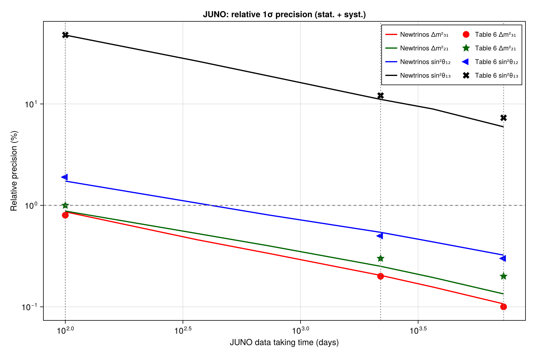
Expected (Asimov) sensitivity of JUNO to Δm²₃₁, Δm²₂₁, sin²θ₁₂ and sin²θ₁₃ in the normal ordering, without an external θ₁₃ constraint, as a function of data-taking time. This is a sensitivity study: there are no data.
Figures
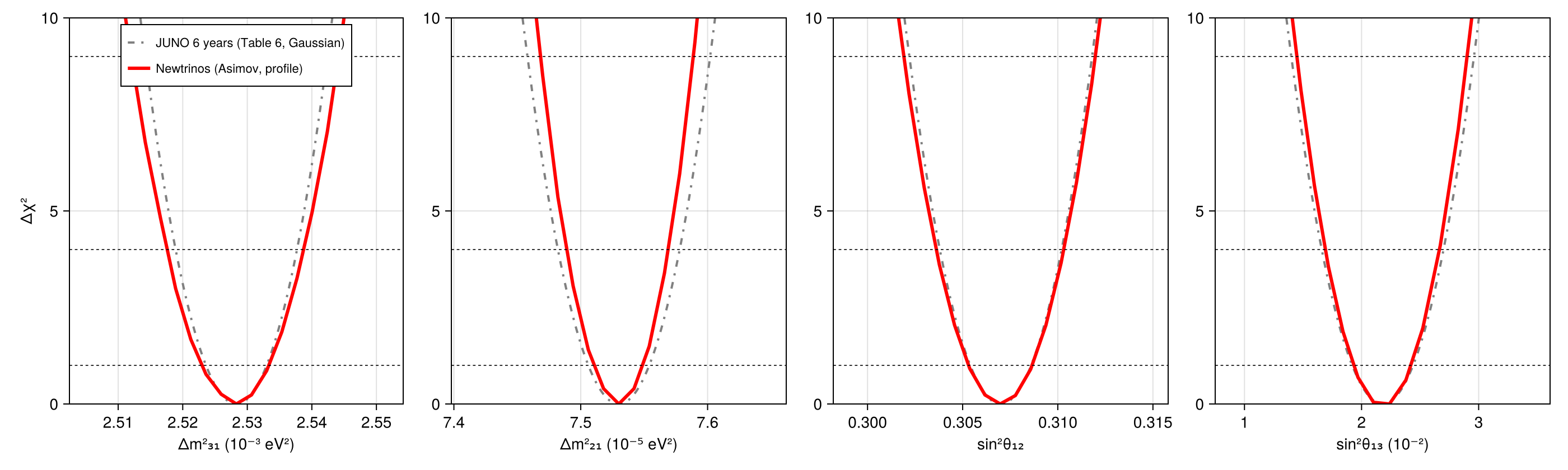
1D Δχ² profiles after 6 years · Fig. 7
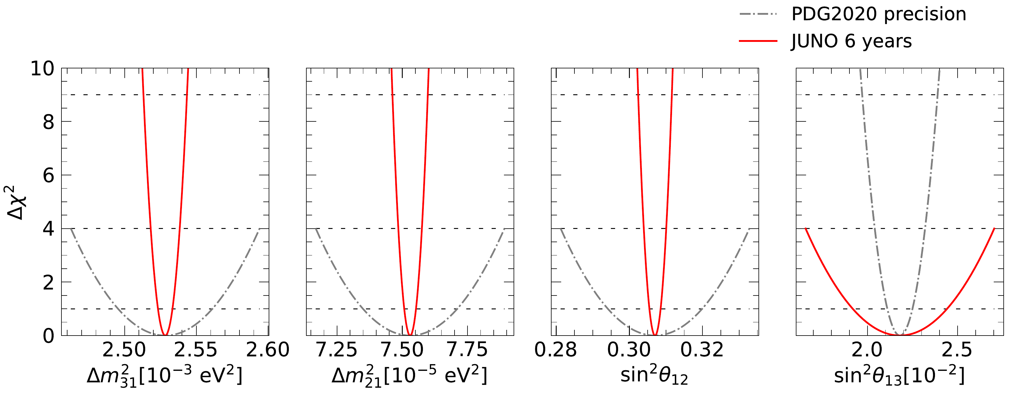
Original figure: JUNO, Chin. Phys. C 46, 123001 (2022), Fig. 7, doi:10.1088/1674-1137/ac8bc9. Not our work; shown for comparison, all rights with the authors and publisher.
Relative precision vs data-taking time · Fig. 8, Table 6
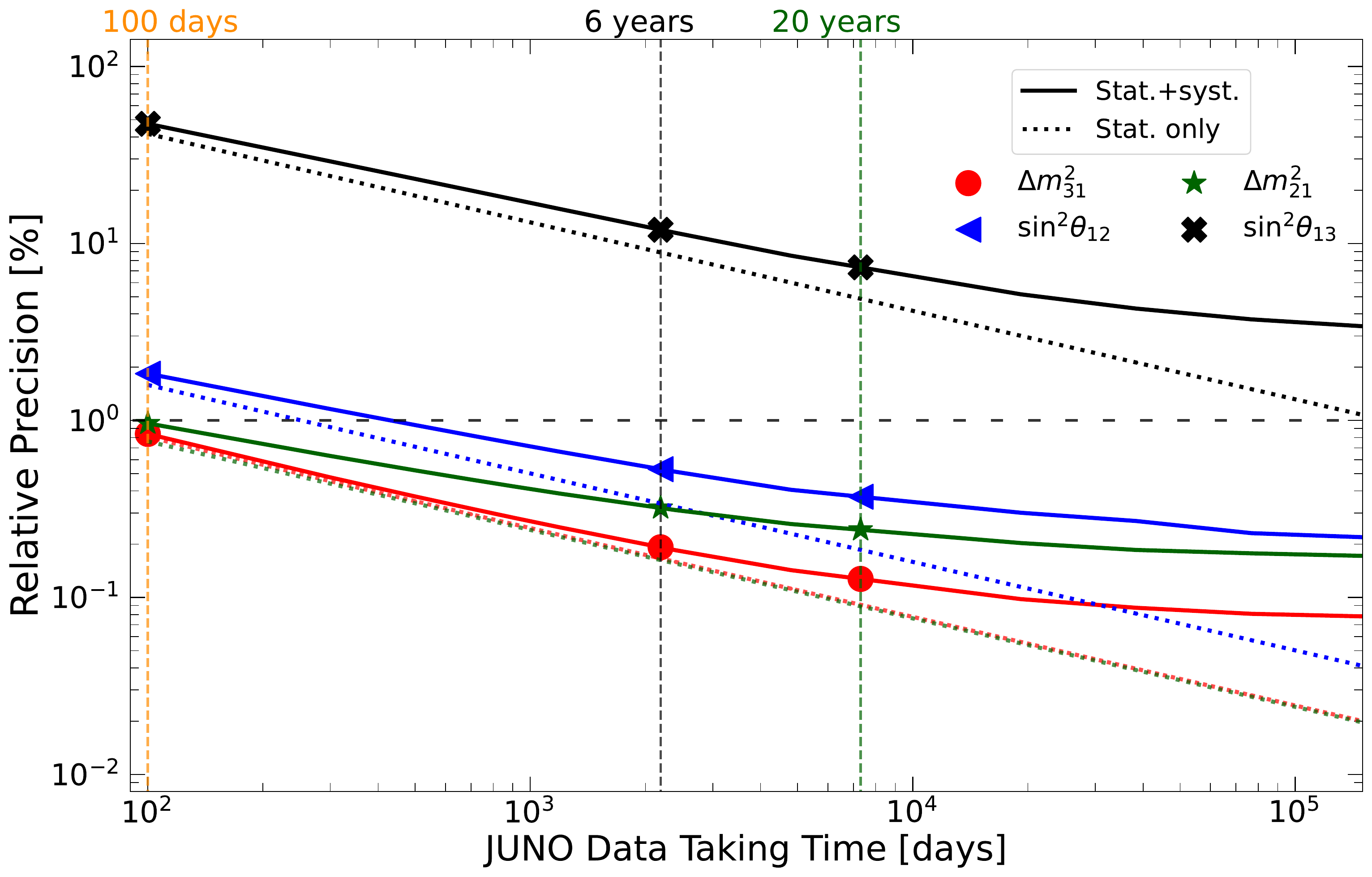
Original figure: JUNO, Chin. Phys. C 46, 123001 (2022), Fig. 8, Table 6, doi:10.1088/1674-1137/ac8bc9. Not our work; shown for comparison, all rights with the authors and publisher.
Known limitations
- Sensitivity reproduction: the Asimov data set at the paper's true point is fitted; the paper's 1σ precisions (Table 6) are compared as Gaussian Δχ² curves and markers.
- The Newtrinos JUNO model (backgrounds, detector response, TAO-constrained reference spectrum) is built from the paper's inputs.
- Agreement within ~10% at 100 days and 6 years except Δm²₂₁ (ours 0.25% vs 0.32% at 6 years); at 20 years our Δm²₂₁ and sin²θ₁₃ precisions (0.13%, 6.0%) are better than the paper's (0.23%, 7.3%), i.e. our systematic floor on the spectral shape is weaker.
Reproduce
git clone https://github.com/Newtrinos-org/Newtrinos.jl.git && cd Newtrinos.jl && git checkout de27463fde- Download reproduce.jl into an empty directory.
julia -t 8 --project=/path/to/Newtrinos.jl reproduce.jl
# Reproduction of JUNO, Chin. Phys. C 46, 123001 (2022) [arXiv:2204.13249], "Sub-percent precision measurement of
# neutrino oscillation parameters with JUNO": Asimov sensitivity with Newtrinos.jl (module `juno`).
# Run from this directory with the Newtrinos.jl environment at the pinned commit:
#   julia -t 8 --project=<path to Newtrinos.jl> reproduce.jl
using Newtrinos, Distributions, DataStructures, Accessors, FileIO, CairoMakie, CSV, DataFrames

cd(@__DIR__); mkpath("ours"); mkpath("results"); mkpath("cache")

# CSV export of a profile scan: one row per grid point, ASCII column names, oscillation parameters in physical
# units (sin²θ, Δm²₃₂ = Δm²₃₁ − Δm²₂₁ in eV², δCP in rad), dchi2 = -2Δlog L w.r.t. `ref` (default: the scan's best fit)
function save_csv(path, r; ref = maximum(r.values.log_posterior))
    ascii(k) = replace(string(k), "θ" => "theta", "Δm²" => "dm2_", "δ" => "d", "₁" => "1", "₂" => "2", "₃" => "3", "CP" => "cp")
    cols = OrderedDict{String,Any}()
    for (k, v) in pairs(r.values)
        x = vec(v)
        if startswith(string(k), "θ")
            cols["sin2_" * ascii(k)] = sin.(x) .^ 2
        elseif k == :Δm²₃₁
            cols["dm2_32"] = x .- vec(r.values.Δm²₂₁)
        end
        cols[ascii(k)] = x
    end
    cols["dchi2"] = 2 .* (ref .- vec(r.values.log_posterior))
    haskey(cols, "llh") && (cols["log_likelihood"] = pop!(cols, "llh"))
    first_cols = filter(in(keys(cols)), ["sin2_theta23", "dm2_32", "dcp", "dchi2", "log_likelihood", "log_posterior"])
    CSV.write(path, DataFrame(cols)[:, vcat(first_cols, setdiff(collect(keys(cols)), first_cols))])
end


# true (Asimov) point of the paper (Table 6, normal ordering); no external constraint on θ₁₃
truth = (Δm²₃₁ = 2.5283e-3, Δm²₂₁ = 7.53e-5, θ₁₂ = asin(sqrt(0.307)), θ₁₃ = asin(sqrt(0.0218)), δCP = 0.0)
# paper's 1σ precision after 6 years (Table 6), used for scan ranges and the comparison
σ6 = (Δm²₃₁ = 0.0047e-3, Δm²₂₁ = 0.024e-5, ss12 = 0.0016, ss13 = 0.0026)
# Table 6 relative precisions [%] at 100 days, 6 years, 20 years
table6 = (days = [100, 6 * 365, 20 * 365], Δm²₃₁ = [0.8, 0.2, 0.1], Δm²₂₁ = [1.0, 0.3, 0.2], ss12 = [1.9, 0.5, 0.3], ss13 = [47.9, 12.1, 7.3])

function sensitivity(years; npoints = 21)
    experiments = (juno = Newtrinos.juno.configure(livetime_years = years),)
    p = merge(Newtrinos.get_params(experiments), truth)
    asimov = Newtrinos.generate_asimov_data(experiments, p)
    likelihood = Newtrinos.generate_likelihood(experiments, asimov)
    priors = merge(Newtrinos.get_priors(experiments), (θ₂₃ = p.θ₂₃, δCP = p.δCP))
    w = 5 * max(1.0, sqrt(6 / years))     # scan ±5 expected σ
    ranges = (Δm²₃₁ = (truth.Δm²₃₁ - w * σ6.Δm²₃₁, truth.Δm²₃₁ + w * σ6.Δm²₃₁),
              Δm²₂₁ = (truth.Δm²₂₁ - w * σ6.Δm²₂₁, truth.Δm²₂₁ + w * σ6.Δm²₂₁),
              θ₁₂ = asin.(sqrt.((0.307 - w * σ6.ss12, 0.307 + w * σ6.ss12))),
              θ₁₃ = asin.(sqrt.((max(0.0218 - w * σ6.ss13, 1e-4), 0.0218 + w * σ6.ss13))))
    # all scans priors must contain the Asimov truth; each scanned parameter gets its own range
    pr_all = merge(priors, map(r -> Uniform(r...), ranges))
    map(keys(ranges)) do v
        cd = "cache/$(round(years, digits = 3))y_$(v)"; mkpath(cd)
        v => Newtrinos.profile(likelihood, pr_all, OrderedDict(v => npoints), p, cache_dir = cd)
    end |> NamedTuple
end

# relative 1σ precision [%] from a 1D profile: half the width of the Δχ² < 1 interval (linear interpolation)
function precision(x, dχ², x0)
    i0 = argmin(dχ²)
    cross(r) = (for i in r[1:end-1]
                    j = r[findfirst(==(i), r) + 1]
                    if (dχ²[i] - 1) * (dχ²[j] - 1) <= 0
                        return x[i] + (1 - dχ²[i]) * (x[j] - x[i]) / (dχ²[j] - dχ²[i])
                    end
                end; NaN)
    lo, hi = cross(collect(i0:-1:1)), cross(collect(i0:length(x)))
    100 * (hi - lo) / 2 / x0
end
dchi2(r) = 2 .* (maximum(r.values.log_posterior) .- r.values.log_posterior)
xvals(v, r) = v == :θ₁₂ || v == :θ₁₃ ? sin.(r.axes[v]) .^ 2 : r.axes[v]
x0(v) = v == :θ₁₂ ? 0.307 : v == :θ₁₃ ? 0.0218 : truth[v]

# --- Fig. 7: 1D Δχ² profiles after 6 years ---
r6 = sensitivity(6.0)
FileIO.save("results/juno_6years.jld2", Dict(string(k) => v for (k, v) in pairs(r6)))
for (k, r) in pairs(r6)
    save_csv("results/juno_6years_$(k).csv", r)
end
panels = ((:Δm²₃₁, "Δm²₃₁ (10⁻³ eV²)", 1e3, σ6.Δm²₃₁), (:Δm²₂₁, "Δm²₂₁ (10⁻⁵ eV²)", 1e5, σ6.Δm²₂₁),
          (:θ₁₂, "sin²θ₁₂", 1.0, σ6.ss12), (:θ₁₃, "sin²θ₁₃ (10⁻²)", 1e2, σ6.ss13))
fig = Figure(size = (1400, 420))
for (i, (v, label, scale, σ)) in enumerate(panels)
    ax = Axis(fig[1, i], xlabel = label, ylabel = i == 1 ? "Δχ²" : "")
    r = r6[v]; x = xvals(v, r)
    xf = range(minimum(x), maximum(x), 200)
    lines!(ax, xf .* scale, ((xf .- x0(v)) ./ σ) .^ 2, color = :gray, linestyle = :dashdot, linewidth = 2, label = "JUNO 6 years (Table 6, Gaussian)")
    lines!(ax, x .* scale, dchi2(r), color = :red, linewidth = 3, label = "Newtrinos (Asimov, profile)")
    hlines!(ax, [1, 4, 9], color = :black, linestyle = :dash, linewidth = 0.8)
    ylims!(ax, 0, 10)
    i == 1 && axislegend(ax, position = :ct, labelsize = 11)
end
save("ours/fig7_dchi2_6years.png", fig)

# --- Fig. 8: relative precision vs data-taking time ---
livetimes = [100 / 365, 1.0, 2.0, 6.0, 10.0, 20.0]
prec = Dict(v => Float64[] for v in (:Δm²₃₁, :Δm²₂₁, :θ₁₂, :θ₁₃))
for y in livetimes
    r = y == 6.0 ? r6 : sensitivity(y)
    for v in keys(prec)
        push!(prec[v], precision(xvals(v, r[v]), dchi2(r[v]), x0(v)))
    end
end
CSV.write("results/juno_precision_vs_time.csv",
          DataFrame(days = livetimes .* 365, dm2_31 = prec[:Δm²₃₁], dm2_21 = prec[:Δm²₂₁], sin2_theta12 = prec[:θ₁₂], sin2_theta13 = prec[:θ₁₃]))
fig = Figure(size = (900, 600))
ax = Axis(fig[1, 1], xscale = log10, yscale = log10, xlabel = "JUNO data taking time (days)", ylabel = "Relative precision (%)",
          title = "JUNO: relative 1σ precision (stat. + syst.)")
for (v, label, c, m) in ((:Δm²₃₁, "Δm²₃₁", :red, :circle), (:Δm²₂₁, "Δm²₂₁", :darkgreen, :star5),
                         (:θ₁₂, "sin²θ₁₂", :blue, :ltriangle), (:θ₁₃, "sin²θ₁₃", :black, :xcross))
    lines!(ax, livetimes .* 365, prec[v], color = c, linewidth = 2, label = "Newtrinos $(label)")
    key = v == :θ₁₂ ? :ss12 : v == :θ₁₃ ? :ss13 : v
    scatter!(ax, table6.days, table6[key], color = c, marker = m, markersize = 16, label = "Table 6 $(label)")
end
hlines!(ax, [1.0], color = :gray, linestyle = :dash)
vlines!(ax, table6.days, color = :gray, linestyle = :dot)
axislegend(ax, position = :rt, nbanks = 2, labelsize = 11)
save("ours/fig8_precision_vs_time.png", fig)
Provenance
| Newtrinos.jl commit | de27463fde (juno) |
|---|---|
| Run date | 2026-10-02T14:00:24Z |
| Wall time | 2.7 min (16 threads) |
| Julia | 1.13.0 |
| Machine | 13th Gen Intel(R) Core(TM) i7-13700H, 20 hardware threads, Linux |
| Environment | newtrinos_Manifest.toml · run.toml |
Downloads
CSV files hold one row per scan point: the scanned and profiled parameters
(sin2_theta23, dm2_32 in eV², dcp in rad, nuisance parameters), dchi2 = −2Δ log L
and the log-likelihood. JLD2 files contain the full NewtrinosResult objects.
| File | Size | SHA-256 |
|---|---|---|
| ours/fig7_dchi2_6years.png | 185.3 kB | 4455bfb1f770… |
| ours/fig8_precision_vs_time.png | 173.9 kB | a8e3b318c72f… |
| results/juno_6years.jld2 | 66.8 kB | d8998ce58ec6… |
| results/juno_6years_Δm²₂₁.csv | 10.8 kB | 04e8d3ffde14… |
| results/juno_6years_Δm²₃₁.csv | 10.9 kB | 7177dd2b0b89… |
| results/juno_6years_θ₁₂.csv | 11.0 kB | d4561b15cea7… |
| results/juno_6years_θ₁₃.csv | 11.0 kB | 44c0f166f338… |
| results/juno_precision_vs_time.csv | 541 B | 13b03aae2cd0… |