
J. N. Bahcall, P. I. Krastev · Phys. Rev. C 56, 2839 (1997)
Does the Sun appear brighter at night in neutrinos?
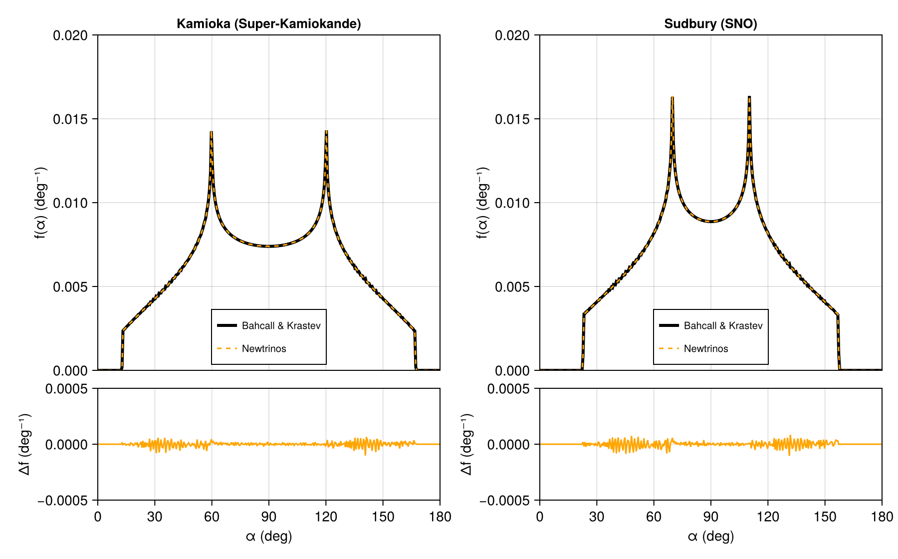
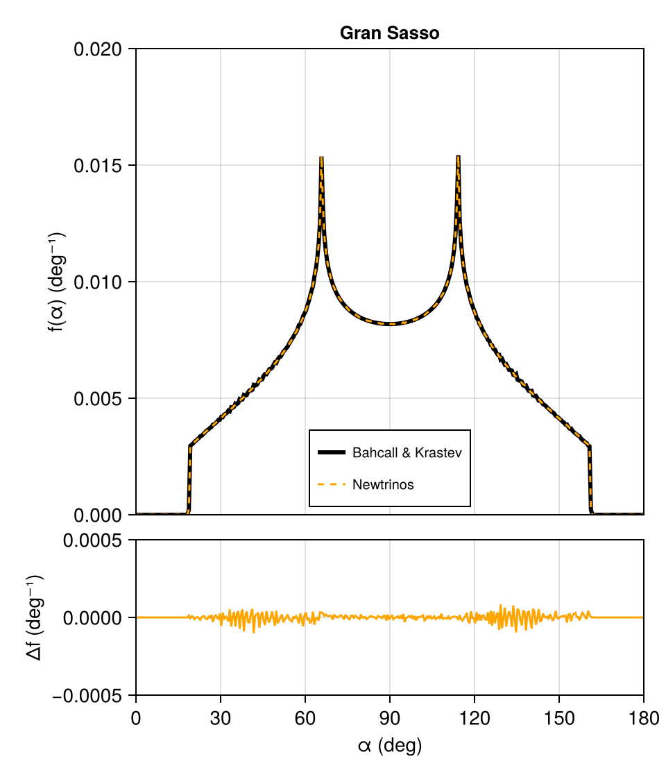
The yearly distribution of the solar zenith angle at a detector, weighted with the Earth–Sun distance (the "zenith-angle exposure function"), which Newtrinos uses for day/night averaging and Earth regeneration of solar neutrinos (solar_flux.nadir_exposure). Compared with Bahcall's tabulation (0.5° bins) for Kamioka (36.4° N), Sudbury (46.3° N) and Gran Sasso (42.4° N), the no-oscillation panels of Figs. 5 and 6: the largest bin-wise difference is 5×10⁻⁵ (0.7 % of the peak bin), the night fraction and the fraction of time behind the Earth's core agree to 10⁻⁴.
Figures
Exposure functions at Kamioka (Super-Kamiokande) and Sudbury (SNO) · Fig. 5 (left)
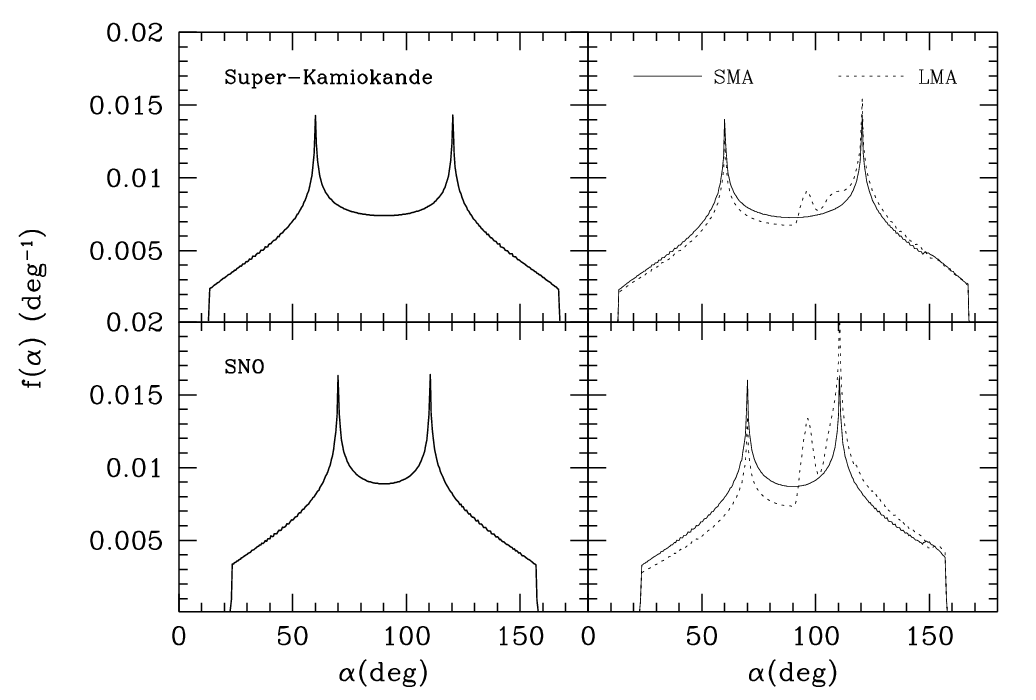
Original figure: J. N. Bahcall, P. I. Krastev, Phys. Rev. C 56, 2839 (1997), Fig. 5 (left), doi:10.1103/PhysRevC.56.2839. Not our work; shown for comparison, all rights with the authors and publisher.
Exposure function at Gran Sasso · Fig. 6 (upper left)
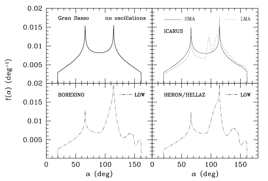
Original figure: J. N. Bahcall, P. I. Krastev, Phys. Rev. C 56, 2839 (1997), Fig. 6 (upper left), doi:10.1103/PhysRevC.56.2839. Not our work; shown for comparison, all rights with the authors and publisher.
Known limitations
- Only the exposure functions (left panels of Fig. 5, upper-left panel of Fig. 6) are compared; the oscillated zenith-angle distributions refer to the SMA, LMA and LOW solutions of 1997.
Reproduce
git clone https://github.com/Newtrinos-org/Newtrinos.jl.git && cd Newtrinos.jl && git checkout c6612c255a- Download reproduce.jl and the
data/folder of this entry into an empty directory. julia -t 8 --project=/path/to/Newtrinos.jl reproduce.jl
# Verification of the Newtrinos.jl solar zenith-angle exposure (`solar_flux.nadir_exposure`) against the exposure
# functions of Bahcall & Krastev, Phys. Rev. C 56, 2839 (1997), Figs. 5 and 6, tabulated by Bahcall in
# data/exposurefunctions (fraction of the year in 0.5° bins of the solar zenith angle, weighted with 1/d²).
# Run from this directory with the Newtrinos.jl environment at the pinned commit:
#   julia --project=<path to Newtrinos.jl> reproduce.jl
using Newtrinos, CairoMakie, CSV, DataFrames, DelimitedFiles, Printf

cd(@__DIR__); mkpath("ours"); mkpath("results")
tab = readdlm("data/exposurefunctions", skipstart = 3)
α = tab[:, 1]                                   # bin centres [deg]
edges = cosd.(reverse(0:0.5:180))               # cos(zenith) bin edges, ascending
sites = (("Kamioka (Super-Kamiokande)", 36.4), ("Sudbury (SNO)", 46.3), ("Gran Sasso", 42.4))
df = DataFrame(zenith_deg = α)
for (k, (name, lat)) in enumerate(sites)
    ours = reverse(Newtrinos.solar_flux.nadir_exposure(lat; cz_edges = edges, n_days = 2000, n_hours = 2880).w)
    ref = tab[:, k + 1] ./ sum(tab[:, k + 1])
    col = split(name)[1]
    df[!, "$(col)_newtrinos"] = ours; df[!, "$(col)_bahcall"] = ref
    @printf("%-28s max |Δ| = %.1e (peak bin %.1e); night fraction %.4f vs %.4f; behind the core (α > 146.8°) %.5f vs %.5f\n",
            name, maximum(abs.(ours .- ref)), maximum(ref), sum(ours[α .> 90]), sum(ref[α .> 90]),
            sum(ours[α .> 146.8]), sum(ref[α .> 146.8]))
end
CSV.write("results/exposure_functions.csv", df)

# f(α) per degree, as plotted in the paper; residuals below
function panel!(fig, j, name)
    col = split(name)[1]
    ax = Axis(fig[1, j], ylabel = "f(α) (deg⁻¹)", title = name, titlesize = 13)
    lines!(ax, α, 2 .* df[!, "$(col)_bahcall"], color = :black, linewidth = 3, label = "Bahcall & Krastev")
    lines!(ax, α, 2 .* df[!, "$(col)_newtrinos"], color = :orange, linewidth = 1.5, linestyle = :dash, label = "Newtrinos")
    xlims!(ax, 0, 180); ylims!(ax, 0, 0.02); hidexdecorations!(ax, grid = false)
    axislegend(ax, position = :cb, labelsize = 10)
    axr = Axis(fig[2, j], xlabel = "α (deg)", ylabel = "Δf (deg⁻¹)")
    lines!(axr, α, 2 .* (df[!, "$(col)_newtrinos"] .- df[!, "$(col)_bahcall"]), color = :orange)
    xlims!(axr, 0, 180); ylims!(axr, -5e-4, 5e-4)
end
fig = Figure(size = (900, 560))
panel!(fig, 1, sites[1][1]); panel!(fig, 2, sites[2][1])
rowsize!(fig.layout, 2, Relative(0.25))
save("ours/fig5_exposure_sk_sno.png", fig)
fig = Figure(size = (480, 560))
panel!(fig, 1, sites[3][1])
rowsize!(fig.layout, 2, Relative(0.25))
save("ours/fig6_exposure_gran_sasso.png", fig)
Provenance
| Newtrinos.jl commit | c6612c255a (solar_flux) |
|---|---|
| Run date | 2026-10-21T16:40:53Z |
| Wall time | 0.9 min (128 threads) |
| Julia | 1.12.5 |
| Machine | AMD EPYC 7702P 64-Core Processor, 128 hardware threads, Linux |
| Environment | newtrinos_Manifest.toml · run.toml |
Downloads
CSV files hold one row per scan point: the scanned and profiled parameters
(sin2_theta23, dm2_32 in eV², dcp in rad, nuisance parameters), dchi2 = −2Δ log L
and the log-likelihood. JLD2 files contain the full NewtrinosResult objects.
| File | Size | SHA-256 |
|---|---|---|
| ours/fig5_exposure_sk_sno.png | 208.8 kB | 48a0bd5c8786… |
| ours/fig6_exposure_gran_sasso.png | 106.1 kB | 4145e055d504… |
| results/exposure_functions.csv | 40.2 kB | 54a5950431a6… |