
W. T. Winter, S. J. Freedman, K. E. Rehm, J. P. Schiffer · Phys. Rev. C 73, 025503 (2006)
The ⁸B neutrino spectrum
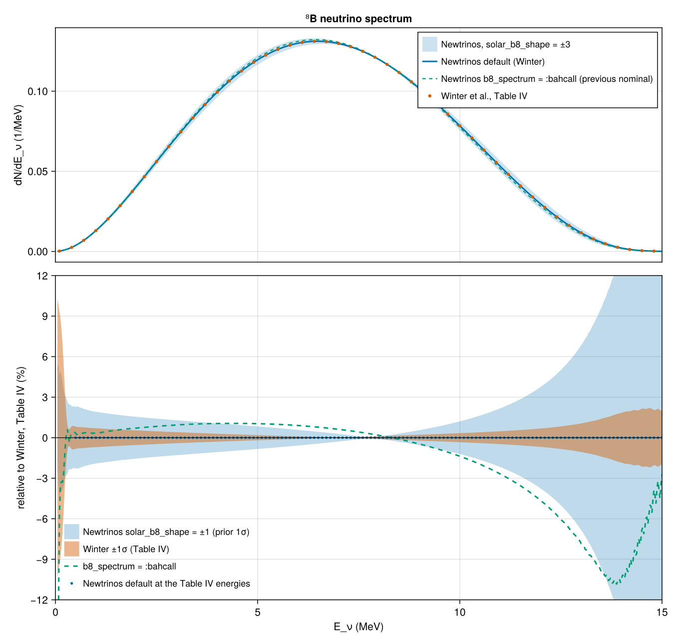
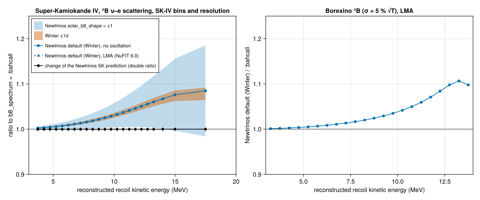
The ⁸B neutrino spectrum deduced by Winter et al. from their measurement of the β-delayed α spectrum (Table IV, recommended by Solar fusion II and used by the Super-Kamiokande and SNO analyses) is the default ⁸B spectrum of Newtrinos' solar_flux module (b8_spectrum = :winter). At the tabulated energies the Newtrinos shape reproduces Table IV to the rounding of the table (results/summary.csv, results/table4_comparison.csv); ⟨E_ν⟩ = 6.770 MeV. The previous nominal, Bahcall et al., Phys. Rev. C 54, 411 (1996) (b8_spectrum = :bahcall, ⟨E_ν⟩ = 6.735 MeV), is shown for comparison: it corresponds to solar_b8_shape ≈ −1 of the new default, whose prior keeps Bahcall's ±3σ variation (Winter's own 1σ is a quarter of it). Compared at the same commit with the same detection physics, Winter's spectrum raises the ⁸B capture rates by about 2.4 % (Cl) and 1.8 % (Ga) and the ν–e scattering rates by about 1.0 % (Super-K IV, 3.5–19.5 MeV) and 0.9 % / 1.5 % (Borexino, T > 3 / 5 MeV), with up to +8 % in the highest Super-K bins. Because the Super-K module normalises to Super-K's own simulation, its prediction changes by less than 5×10⁻⁴; the SNO module does not use the spectrum.
Figures
⁸B spectrum: Newtrinos default vs Winter et al., Table IV (with its ±1σ and the solar_b8_shape prior), and the previous Bahcall (1996) nominal · Fig. 12 (top) and Table IV
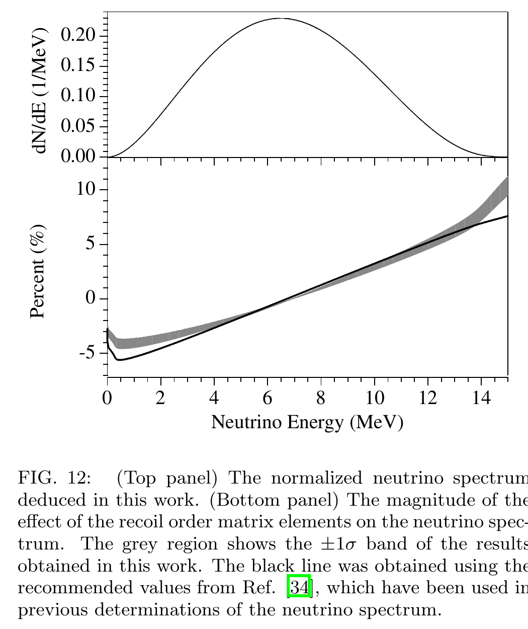
Original figure: W. T. Winter, S. J. Freedman, K. E. Rehm, J. P. Schiffer, Phys. Rev. C 73, 025503 (2006), Fig. 12 (top) and Table IV, doi:10.1103/PhysRevC.73.025503. Not our work; shown for comparison, all rights with the authors and publisher.
Winter vs Bahcall nominal in the ν–e scattering spectra: Super-K IV bins (no oscillation, LMA, and the change of the Newtrinos Super-K prediction) and Borexino ⁸B · —
—
Known limitations
- The detector numbers compare
b8_spectrum = :winterand:bahcallat the pinned commit with identical detection physics (results/rates.csv, results/sk4_bins.csv), so they isolate the change of the ⁸B spectrum from the other solar changes of that commit (QED corrections of ν–e scattering, level-crossing probability). - Winter's ±1σ (ΔP column) is fully correlated and changes sign at 6.85 MeV; it covers the α-spectrum and recoil-order (weak magnetism) uncertainties. Later α-spectrum measurements (Kirsebom et al. 2011, Roger et al. 2012, Longfellow et al. 2023) put the α peak about 20 keV lower and differ from Winter's neutrino spectrum by up to ≈5 % below 15 MeV; Solar fusion III (Rev. Mod. Phys. 97, 035002, Sec. II.D.3) now recommends Longfellow et al. (2023), with Winter et al. as the alternative. Longfellow's tabulated spectrum is not public on arXiv and is not compared here.
- Table IV was transcribed from the arXiv version (data/winter_table4.csv; original/table4.png is the table); it sums to 999.98 per 1000 and ends at 15.2 MeV. Newtrinos interpolates it with cubic splines on Bahcall's 0.02 MeV grid, renormalises it to 1 and continues it above 15.2 MeV with Bahcall's shape (1.1×10⁻⁵ of the flux); the reference curve of this entry is an independent cubic spline of the table. The wiggles of the ratios below 0.5 MeV and above 14 MeV come from the rounding of Winter's table and the point-to-point fluctuations (1–2 %) of Bahcall's tabulated spectrum, whose ±3σ differences also define the
solar_b8_shapevariation. - Detector predictions use Newtrinos' detection physics (ν–e scattering with radiative corrections, ³⁷Cl and ⁷¹Ga cross sections), Gaussian resolutions (SK-IV: that of the sk4_solar module and its bins; Borexino: 5 %/√T) and the NuFIT 6.0 solar parameters (sin²θ₁₂ = 0.308, Δm²₂₁ = 7.49×10⁻⁵ eV², day–night averaged). The Super-K module scales Super-K's simulated rates (made with Winter's spectrum) by the ratio of the Newtrinos prediction to its value at the nominal shape without oscillations, so only the double ratio shown in the figure changes its prediction.
- The Cl and Ga absorption cross-section tables are Bahcall's; Bahcall's spectrum-averaged ⁸B cross section on ³⁷Cl (1.14×10⁻⁴² cm²) becomes 1.169×10⁻⁴² cm² with Winter's spectrum.
Reproduce
git clone https://github.com/Newtrinos-org/Newtrinos.jl.git && cd Newtrinos.jl && git checkout aa98e0c218- Download reproduce.jl and the
data/folder of this entry into an empty directory. julia -t 8 --project=/path/to/Newtrinos.jl reproduce.jl
# Verification of the ⁸B neutrino spectrum of Newtrinos.jl (module `solar_flux`, default `b8_spectrum = :winter`) against
# W. T. Winter et al., Phys. Rev. C 73, 025503 (2006), Table IV (data/winter_table4.csv), with the previous nominal
# (Bahcall et al., PRC 54, 411 (1996), `b8_spectrum = :bahcall`) for comparison, and the effect of the change on the
# predictions for Super-Kamiokande IV, Borexino (⁸B), Homestake and the gallium experiments.
# Run from this directory with the Newtrinos.jl environment at the pinned commit:
#   julia --project=<path to Newtrinos.jl> reproduce.jl
using Newtrinos, CairoMakie, DelimitedFiles, Interpolations, Printf

cd(@__DIR__); mkpath("ours"); mkpath("results")

const SF = Newtrinos.solar_flux
const SC = Newtrinos.solar_common

# ------------------------------------------------------------------------------------------------
# spectral shapes, normalised to 1 per MeV
# ------------------------------------------------------------------------------------------------
sfN = SF.configure()                                                    # default: Winter et al. 2006
sfB = SF.configure(SF.SolarFluxConfig(b8_spectrum = :bahcall))          # previous nominal: Bahcall et al. 1996
@assert sfN.cfg.b8_spectrum == :winter
shape(sf, E, s) = sf.spectrum(:b8, E, merge(sf.params, (solar_b8_shape = s,))) ./ sf.flux(:b8, sf.params)
fN(E, s = 0.0) = shape(sfN, E, s)                                       # Newtrinos (vectorised in E)
fB(E, s = 0.0) = shape(sfB, E, s)                                       # Newtrinos, b8_spectrum = :bahcall

# Winter et al., Table IV: independent cubic spline on the 0.1 MeV grid of the table (normalised to 1000 per MeV)
w = readdlm("data/winter_table4.csv", ',', Float64; skipstart = 3)
const Ew, Pw, dPw = w[:, 1], w[:, 2] ./ 1000, w[:, 3] ./ 1000
@assert Ew ≈ 0.1:0.1:15.5
itpW = cubic_spline_interpolation(0.0:0.1:15.5, vcat(0.0, Pw), extrapolation_bc = 0.0)
itpdW = cubic_spline_interpolation(0.0:0.1:15.5, vcat(0.0, dPw), extrapolation_bc = 0.0)
fW(E, s = 0.0) = [e > 15.2 ? 0.0 : max(itpW(e) + s * itpdW(e), 0.0) for e in E]   # s = ±1: Winter's ±1σ (ΔP > 0 at low E: softer)

const G = collect(0.0:0.005:16.6)
trapz(y) = sum((y[1:end-1] .+ y[2:end]) ./ 2) * step(0.0:0.005:16.6)
meanE(y) = trapz(G .* y) / trapz(y)

# --- 1. Newtrinos default vs Table IV at the tabulated energies ---
tab = (Ew .>= 0.5) .& (Ew .<= 15.0)
rel_tab = fN(Ew[tab]) ./ Pw[tab] .- 1
big = abs.(dPw[tab]) .>= 0.01e-3                          # |ΔP| ≥ 0.01 per 1000: away from the sign change at 6.85 MeV
pull_tab = (fN(Ew[tab]) .- Pw[tab]) ./ abs.(dPw[tab])
EN, EB, EW = meanE(fN(G)), meanE(fB(G)), meanE(fW(G))
EWp, EWm = meanE(fW(G, 1.0)), meanE(fW(G, -1.0))
dEds = meanE(fN(G, 1.0)) - EN                             # change of ⟨E⟩ per unit of solar_b8_shape
@printf("normalisation: Newtrinos %.6f, Table IV %.6f\n", trapz(fN(G)), trapz(fW(G)))
@printf("Newtrinos default vs Table IV at the tabulated energies 0.5–15 MeV: max |rel. dev.| %.2e (2–13 MeV: %.2e); max |Δ|/|ΔP| = %.3f where |ΔP| ≥ 0.01\n",
        maximum(abs.(rel_tab)), maximum(abs.(rel_tab[2 .<= Ew[tab] .<= 13])), maximum(abs.(pull_tab[big])))
@printf("<E>: Newtrinos %.4f MeV, Table IV %.4f MeV (+1σ %.4f, -1σ %.4f), Bahcall (b8_spectrum = :bahcall) %.4f MeV\n", EN, EW, EWp, EWm, EB)
σW_in_s = (EWm - EWp) / 2 / dEds
s_bahcall = (EB - EN) / dEds
mask = (G .>= 0.1) .& (G .<= 15.0)
gN = (fN(G, 1.0) .- fN(G)) .* mask
s_bahcall_lsq = sum((fB(G) .- fN(G)) .* gN) / sum(gN .^ 2)
res_B = maximum(abs.(fN(G, s_bahcall_lsq) ./ fB(G) .- 1)[(G .>= 2) .& (G .<= 13)])
dev_B = maximum(abs.(fW(G) ./ fB(G) .- 1)[(G .>= 2) .& (G .<= 13)])
@printf("Winter's 1σ = %.3f σ of solar_b8_shape; Bahcall's best estimate ≙ solar_b8_shape = %+.3f (<E>), %+.3f (least squares, max rel. residual 2–13 MeV %.4f)\n",
        σW_in_s, s_bahcall, s_bahcall_lsq, res_B)
@printf("max |Winter/Bahcall - 1| over 2–13 MeV: %.4f\n", dev_B)

# ------------------------------------------------------------------------------------------------
# 2. detector predictions: Newtrinos default (Winter) vs b8_spectrum = :bahcall, same commit and detection physics
# ------------------------------------------------------------------------------------------------
physics = SC.default_physics()
xs = physics.solar_xsec
# NuFIT 6.0 (IC19 w/o SK-atm) best fit for the solar parameters
p = merge(physics.osc.params, sfN.params, xs.params,
          (θ₁₂ = asin(sqrt(0.308)), θ₁₃ = asin(sqrt(0.02215)), Δm²₂₁ = 7.49e-5))
Φ = sfN.nominal.b8
shapes = [("Bahcall (b8_spectrum = :bahcall)", E -> fB(E)),
          ("Newtrinos default (Winter)", E -> fN(E)),
          ("Newtrinos default, s = +1", E -> fN(E, 1.0)), ("Newtrinos default, s = -1", E -> fN(E, -1.0)),
          ("Winter Table IV +1σ", E -> fW(E, 1.0)), ("Winter Table IV -1σ", E -> fW(E, -1.0))]

# radiochemical: ⁸B capture rate [SNU]
function capture(target, thr, lat, depth, f; osc = true)
    site = SC.Site(physics, lat; depth_km = depth)
    E = collect(range(thr, 16.6, length = 400)); wE = SC.trapezoid_weights(E)
    P = osc ? SC.averaged_prob(physics, site, :b8, E, p)[:, 1] : ones(length(E))
    sum(wE .* Φ .* f(E) .* P .* [xs.capture(target, e, p) for e in E]) / 1e-36
end
# elastic scattering: rate per reconstructed kinetic-energy bin [events per target electron per s]
function es(resp, site, f; osc = true)
    P = osc ? SC.averaged_prob(physics, site, :b8, resp.E, p)[:, 1] : ones(length(resp.E))
    SC.es_rates(resp, Φ .* f(resp.E), P)
end
Enu = collect(range(2.0, 16.6, length = 220))
# Super-Kamiokande IV: analysis bins and resolution of Newtrinos.sk4_solar
skcsv = readdlm(joinpath(pkgdir(Newtrinos), "src/experiments/super_k/sk_solar_iv_2970d/sk4_solar_spectrum.csv"), ',', Any, '\n';
                comments = true, header = true)[1]
skbins = unique(collect(zip(Float64.(skcsv[:, 1]), Float64.(skcsv[:, 2]))))
sk_res(E) = -0.0839 + 0.349 * sqrt(E) + 0.0397 * E
sk_site = SC.Site(physics, 36.43; depth_km = 1.0)
resp_sk = SC.ESResponse(xs, Enu, skbins, sk_res; scale_unc = 0.0048, reso_unc = 0.03)
resp_sk_tot = SC.ESResponse(xs, Enu, [(3.49, 19.49)], sk_res; scale_unc = 0.0048, reso_unc = 0.03)
# Borexino: σ = 5 % √(T/MeV), as in Newtrinos.borexino_ph1_spectrum; T > 3 MeV and T > 5 MeV
bx_res(E) = 0.05 * sqrt(max(E - Newtrinos.solar_xsec.M_E, 1e-3))
bx_site = SC.Site(physics, 42.45; depth_km = 1.4)
bxbins = [(t, t + 0.5) for t in 3.0:0.5:13.5]
resp_bx = SC.ESResponse(xs, Enu, bxbins, bx_res; scale_unc = 0.01, reso_unc = 0.1)
resp_bx_tot = SC.ESResponse(xs, Enu, [(3.0, 20.0), (5.0, 20.0)], bx_res; scale_unc = 0.01, reso_unc = 0.1)

rows = []
for (name, f) in shapes
    cl = (capture(:cl37, Newtrinos.solar_xsec.CL_THRESHOLD, 44.35, 1.48, f; osc = false), capture(:cl37, Newtrinos.solar_xsec.CL_THRESHOLD, 44.35, 1.48, f))
    ga = (capture(:ga71, Newtrinos.solar_xsec.GA_THRESHOLD, 42.45, 1.4, f; osc = false), capture(:ga71, Newtrinos.solar_xsec.GA_THRESHOLD, 42.45, 1.4, f))
    sk = (es(resp_sk_tot, sk_site, f; osc = false)[1], es(resp_sk_tot, sk_site, f)[1])
    bx = (es(resp_bx_tot, bx_site, f; osc = false), es(resp_bx_tot, bx_site, f))
    push!(rows, (; name, cl, ga, sk, bx3 = (bx[1][1], bx[2][1]), bx5 = (bx[1][2], bx[2][2]), meanE = meanE(f(G))))
end
ref = rows[1]
open("results/rates.csv", "w") do io
    println(io, "# ⁸B predictions relative to b8_spectrum = :bahcall (the previous nominal), same Newtrinos commit and detection physics;")
    println(io, "# no oscillation and NuFIT 6.0 LMA (day+night). Cl, Ga: capture rate; SK-IV: ES rate in 3.49–19.49 MeV (kinetic, reconstructed);")
    println(io, "# Borexino: ES rate T > 3 and > 5 MeV. Absolute values for :bahcall, LMA: Cl ⁸B $(round(ref.cl[2], digits = 4)) SNU, Ga ⁸B $(round(ref.ga[2], digits = 4)) SNU")
    println(io, "shape,mean_E_MeV,Cl_noosc,Cl_osc,Ga_noosc,Ga_osc,SK4_noosc,SK4_osc,BX3_noosc,BX3_osc,BX5_noosc,BX5_osc")
    for r in rows
        q = collect(Iterators.flatten((r.cl ./ ref.cl, r.ga ./ ref.ga, r.sk ./ ref.sk, r.bx3 ./ ref.bx3, r.bx5 ./ ref.bx5)))
        println(io, "\"$(r.name)\",", @sprintf("%.4f", r.meanE), ",", join([@sprintf("%.5f", x) for x in q], ","))
    end
end
@printf("Newtrinos default (Winter), NuFIT 6.0 LMA: Cl ⁸B %.3f SNU, Ga ⁸B %.3f SNU\n", rows[2].cl[2], rows[2].ga[2])
println("ratios to b8_spectrum = :bahcall (no osc / LMA):")
for r in rows[2:end]
    @printf("  %-28s Cl %.4f/%.4f  Ga %.4f/%.4f  SK-IV %.4f/%.4f  BX(T>3) %.4f/%.4f  BX(T>5) %.4f/%.4f\n", r.name,
            (r.cl ./ ref.cl)..., (r.ga ./ ref.ga)..., (r.sk ./ ref.sk)..., (r.bx3 ./ ref.bx3)..., (r.bx5 ./ ref.bx5)...)
end

# SK-IV per bin. Newtrinos.sk4_solar normalises its rates to SK's MC (mc_b8) times spectrum(params)/spectrum(nominal) at
# P_ee = 1, so what the change of the nominal shape changes in the SK prediction is the double ratio
# [R(osc)/R(no osc)]_Winter / [R(osc)/R(no osc)]_Bahcall.
skW = (es(resp_sk, sk_site, E -> fN(E); osc = false), es(resp_sk, sk_site, E -> fN(E)))
skB = (es(resp_sk, sk_site, E -> fB(E); osc = false), es(resp_sk, sk_site, E -> fB(E)))
skNp = es(resp_sk, sk_site, E -> fN(E, 1.0); osc = false); skNm = es(resp_sk, sk_site, E -> fN(E, -1.0); osc = false)
skWp = es(resp_sk, sk_site, E -> fW(E, 1.0); osc = false); skWm = es(resp_sk, sk_site, E -> fW(E, -1.0); osc = false)
dbl = (skW[2] ./ skW[1]) ./ (skB[2] ./ skB[1])
bxW = es(resp_bx, bx_site, E -> fN(E)); bxB = es(resp_bx, bx_site, E -> fB(E))
open("results/sk4_bins.csv", "w") do io
    println(io, "# SK-IV bins, ratios to b8_spectrum = :bahcall without oscillation unless noted; double_ratio = change of the Newtrinos SK prediction")
    println(io, "T_lo,T_hi,newtrinos_over_bahcall_noosc,newtrinos_over_bahcall_osc,newtrinos_plus1_over_bahcall,newtrinos_minus1_over_bahcall,winter_plus1sigma_over_bahcall,winter_minus1sigma_over_bahcall,double_ratio")
    for k in eachindex(skbins)
        println(io, join([skbins[k]..., skW[1][k] / skB[1][k], skW[2][k] / skB[2][k], skNp[k] / skB[1][k], skNm[k] / skB[1][k],
                          skWp[k] / skB[1][k], skWm[k] / skB[1][k], dbl[k]], ","))
    end
end
@printf("SK-IV bins: Newtrinos/Bahcall (no osc) from %.4f to %.4f; double ratio (change of the Newtrinos SK prediction) %.5f to %.5f\n",
        extrema(skW[1] ./ skB[1])..., extrema(dbl)...)

# ------------------------------------------------------------------------------------------------
# tables and figures
# ------------------------------------------------------------------------------------------------
open("results/table4_comparison.csv", "w") do io
    println(io, "# Newtrinos default ⁸B shape at the energies of Winter et al., Table IV (both per 1000 per MeV)")
    println(io, "E,table_P,table_DeltaP,newtrinos,newtrinos_minus_table")
    for (e, P, d, n) in zip(Ew, Pw .* 1000, dPw .* 1000, fN(Ew) .* 1000)
        println(io, join([@sprintf("%.2f", e), @sprintf("%.3f", P), @sprintf("%.3f", d), @sprintf("%.4f", n), @sprintf("%.4f", n - P)], ","))
    end
end
Et = collect(0.1:0.1:16.5)
open("results/shape.csv", "w") do io
    println(io, "# normalised ⁸B spectra [1/MeV]: Newtrinos default (Winter) with solar_b8_shape s, b8_spectrum = :bahcall, Winter Table IV (cubic spline)")
    println(io, "E,newtrinos_s0,newtrinos_s_plus1,newtrinos_s_minus1,bahcall,table4,table4_plus1sigma,table4_minus1sigma")
    for (i, e) in enumerate(Et)
        vals = (fN(Et)[i], fN(Et, 1.0)[i], fN(Et, -1.0)[i], fB(Et)[i], fW(Et)[i], fW(Et, 1.0)[i], fW(Et, -1.0)[i])
        println(io, join([@sprintf("%.2f", e); [@sprintf("%.6e", x) for x in vals]], ","))
    end
end
open("results/summary.csv", "w") do io
    println(io, "quantity,value")
    for (k, v) in (("max_rel_dev_newtrinos_table4_0p5_15MeV", maximum(abs.(rel_tab))),
                   ("max_rel_dev_newtrinos_table4_2_13MeV", maximum(abs.(rel_tab[2 .<= Ew[tab] .<= 13]))),
                   ("max_abs_dev_over_DeltaP_where_DeltaP_ge_0p01", maximum(abs.(pull_tab[big]))),
                   ("mean_E_newtrinos_MeV", EN), ("mean_E_table4_MeV", EW), ("mean_E_bahcall_MeV", EB),
                   ("dmeanE_per_solar_b8_shape_MeV", dEds), ("winter_1sigma_in_solar_b8_shape_units", σW_in_s),
                   ("bahcall_as_solar_b8_shape_meanE", s_bahcall), ("bahcall_as_solar_b8_shape_lsq", s_bahcall_lsq),
                   ("max_rel_residual_newtrinos_slsq_vs_bahcall_2_13MeV", res_B), ("max_rel_dev_winter_bahcall_2_13MeV", dev_B))
        println(io, k, ",", @sprintf("%.5g", v))
    end
end

c_new, c_tab, c_old = Makie.wong_colors()[1], Makie.wong_colors()[6], Makie.wong_colors()[3]
Ep = collect(0.05:0.025:15.0)
fig = Figure(size = (900, 860))
ax1 = Axis(fig[1, 1], ylabel = "dN/dE_ν (1/MeV)", title = "⁸B neutrino spectrum")
band!(ax1, Ep, fN(Ep, -3.0), fN(Ep, 3.0), color = (c_new, 0.2), label = "Newtrinos, solar_b8_shape = ±3")
lines!(ax1, Ep, fN(Ep), color = c_new, linewidth = 2, label = "Newtrinos default (Winter)")
lines!(ax1, Ep, fB(Ep), color = c_old, linewidth = 1.5, linestyle = :dash, label = "Newtrinos b8_spectrum = :bahcall (previous nominal)")
scatter!(ax1, Ew[1:3:end], Pw[1:3:end], color = c_tab, markersize = 6, label = "Winter et al., Table IV")
axislegend(ax1, position = :rt, labelsize = 12)
hidexdecorations!(ax1, grid = false)
ax2 = Axis(fig[2, 1], xlabel = "E_ν (MeV)", ylabel = "relative to Winter, Table IV (%)")
rel(y) = 100 .* (y ./ fW(Ep) .- 1)
band!(ax2, Ep, rel(fN(Ep, -1.0)), rel(fN(Ep, 1.0)), color = (c_new, 0.25), label = "Newtrinos solar_b8_shape = ±1 (prior 1σ)")
band!(ax2, Ep, rel(fW(Ep, -1.0)), rel(fW(Ep, 1.0)), color = (c_tab, 0.45), label = "Winter ±1σ (Table IV)")
lines!(ax2, Ep, rel(fB(Ep)), color = c_old, linewidth = 2, linestyle = :dash, label = "b8_spectrum = :bahcall")
scatter!(ax2, Ew[tab], 100 .* rel_tab, color = c_new, markersize = 5, label = "Newtrinos default at the Table IV energies")
hlines!(ax2, [0.0], color = :black, linewidth = 0.8)
ylims!(ax2, -12, 12); xlims!(ax2, 0, 15); xlims!(ax1, 0, 15)
axislegend(ax2, position = :lb, framevisible = false, labelsize = 12)
linkxaxes!(ax1, ax2)
rowsize!(fig.layout, 1, Relative(0.42))
save("ours/spectrum.png", fig, px_per_unit = 1.5)

fig = Figure(size = (1100, 460))
mid(b) = [(lo + hi) / 2 for (lo, hi) in b]
ax = Axis(fig[1, 1], xlabel = "reconstructed recoil kinetic energy (MeV)", ylabel = "ratio to b8_spectrum = :bahcall",
          title = "Super-Kamiokande IV, ⁸B ν–e scattering, SK-IV bins and resolution")
xs_sk = mid(skbins)
band!(ax, xs_sk, skNm ./ skB[1], skNp ./ skB[1], color = (c_new, 0.25), label = "Newtrinos solar_b8_shape = ±1")
band!(ax, xs_sk, skWm ./ skB[1], skWp ./ skB[1], color = (c_tab, 0.45), label = "Winter ±1σ")
scatterlines!(ax, xs_sk, skW[1] ./ skB[1], color = c_new, label = "Newtrinos default (Winter), no oscillation")
scatterlines!(ax, xs_sk, skW[2] ./ skB[2], color = c_new, marker = :utriangle, linestyle = :dash, label = "Newtrinos default (Winter), LMA (NuFIT 6.0)")
scatterlines!(ax, xs_sk, dbl, color = :black, marker = :diamond, label = "change of the Newtrinos SK prediction (double ratio)")
hlines!(ax, [1.0], color = :black, linewidth = 0.8)
ylims!(ax, 0.9, 1.25); xlims!(ax, 3, 20)
axislegend(ax, position = :lt, labelsize = 11)
ax = Axis(fig[1, 2], xlabel = "reconstructed recoil kinetic energy (MeV)", ylabel = "Newtrinos default (Winter) / :bahcall",
          title = "Borexino ⁸B (σ = 5 % √T), LMA")
scatterlines!(ax, mid(bxbins), bxW ./ bxB, color = c_new)
hlines!(ax, [1.0], color = :black, linewidth = 0.8)
ylims!(ax, 0.9, 1.25); xlims!(ax, 3, 14)
save("ours/detectors.png", fig, px_per_unit = 1.5)
println("done")
Provenance
| Newtrinos.jl commit | aa98e0c218 (solar_flux (b8_spectrum = :winter, :bahcall), solar_xsec, solar_common, sk4_solar (bins, resolution)) |
|---|---|
| Run date | 2026-10-13T12:09:39Z |
| Wall time | 1.6 min (8 threads) |
| Julia | 1.12.5 |
| Machine | AMD EPYC 7702P 64-Core Processor, 128 hardware threads, Linux |
| Environment | newtrinos_Manifest.toml · run.toml |
Downloads
CSV files hold one row per scan point: the scanned and profiled parameters
(sin2_theta23, dm2_32 in eV², dcp in rad, nuisance parameters), dchi2 = −2Δ log L
and the log-likelihood. JLD2 files contain the full NewtrinosResult objects.
| File | Size | SHA-256 |
|---|---|---|
| ours/detectors.png | 141.5 kB | 96c08dcaad33… |
| ours/spectrum.png | 188.6 kB | affe0a27474c… |
| results/rates.csv | 1.1 kB | d0ea90717211… |
| results/shape.csv | 15.8 kB | 47e1c2418f8e… |
| results/sk4_bins.csv | 3.5 kB | 8504275e02f3… |
| results/summary.csv | 512 B | 8273696c15f5… |
| results/table4_comparison.csv | 5.5 kB | 9a83f9875267… |