
SNO · Phys. Rev. C 88, 025501 (2013)
Combined Analysis of all Three Phases of Solar Neutrino Data from the Sudbury Neutrino Observatory
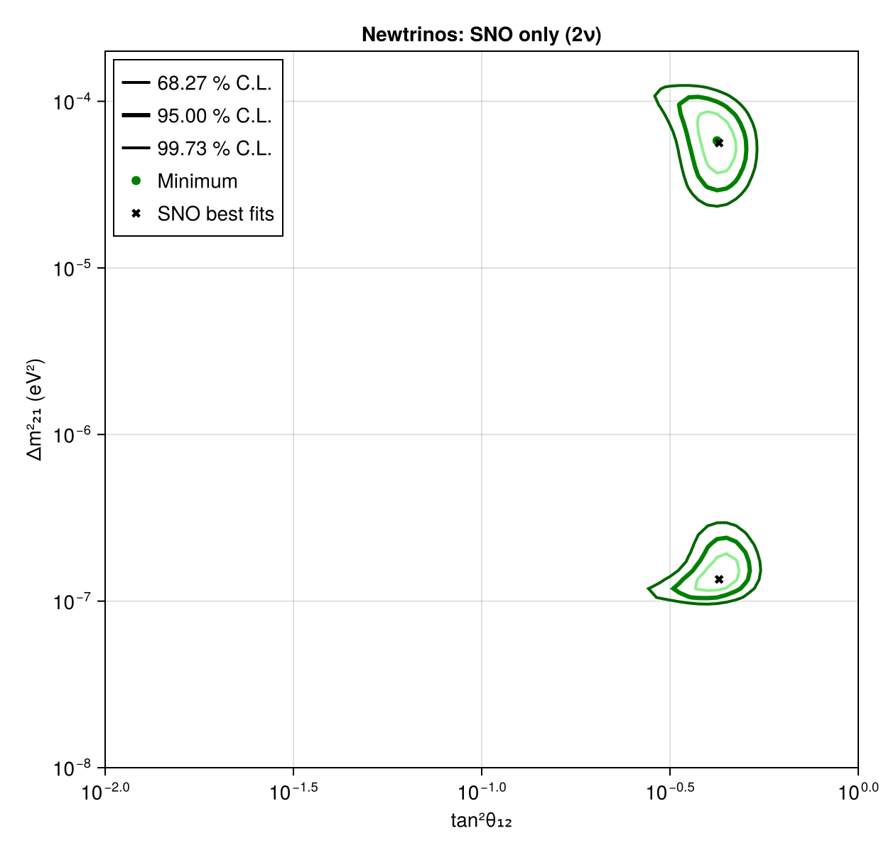
SNO summarises all three phases by the total ⁸B flux, a quadratic day-time νe survival probability and a linear day/night asymmetry in E_ν (Tables X–XI). The Newtrinos sno module compares a model with these numbers following SNO's prescription (projecting the model's day and night probabilities onto the polynomials with the detector sensitivity S(E_ν) tabulated in the paper). With two flavours and a free ⁸B flux, the SNO-only LMA region of Fig. 14 is reproduced: tan²θ₁₂ = 0.422 [0.398, 0.447], Δm²₂₁ = 5.8 [4.5, 7.4]×10⁻⁵ eV², χ²/ndf = 1.55/3 (SNO: 0.427 [0.398, 0.460], 5.62 [4.26, 7.54]×10⁻⁵ eV², 1.39/3), and so is the LOW island, which closes thanks to the non-adiabatic conversion in the Sun: Δm²₂₁ = 1.35×10⁻⁷ eV², χ²/ndf = 1.57/3 (SNO: 1.35 +0.35/−0.14 ×10⁻⁷ eV², 1.41/3).
Figures
SNO-only two-flavour (tan²θ₁₂, Δm²₂₁) regions · Fig. 14
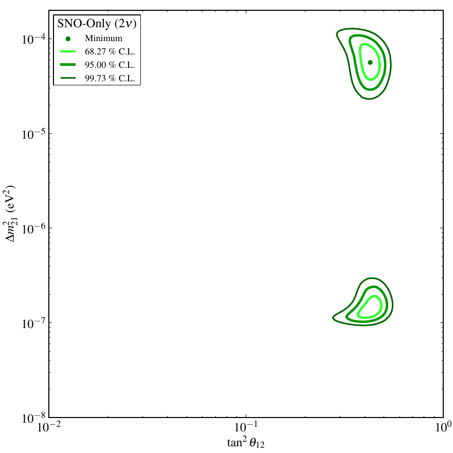
Original figure: SNO, Phys. Rev. C 88, 025501 (2013), Fig. 14, doi:10.1103/PhysRevC.88.025501. Not our work; shown for comparison, all rights with the authors and publisher.
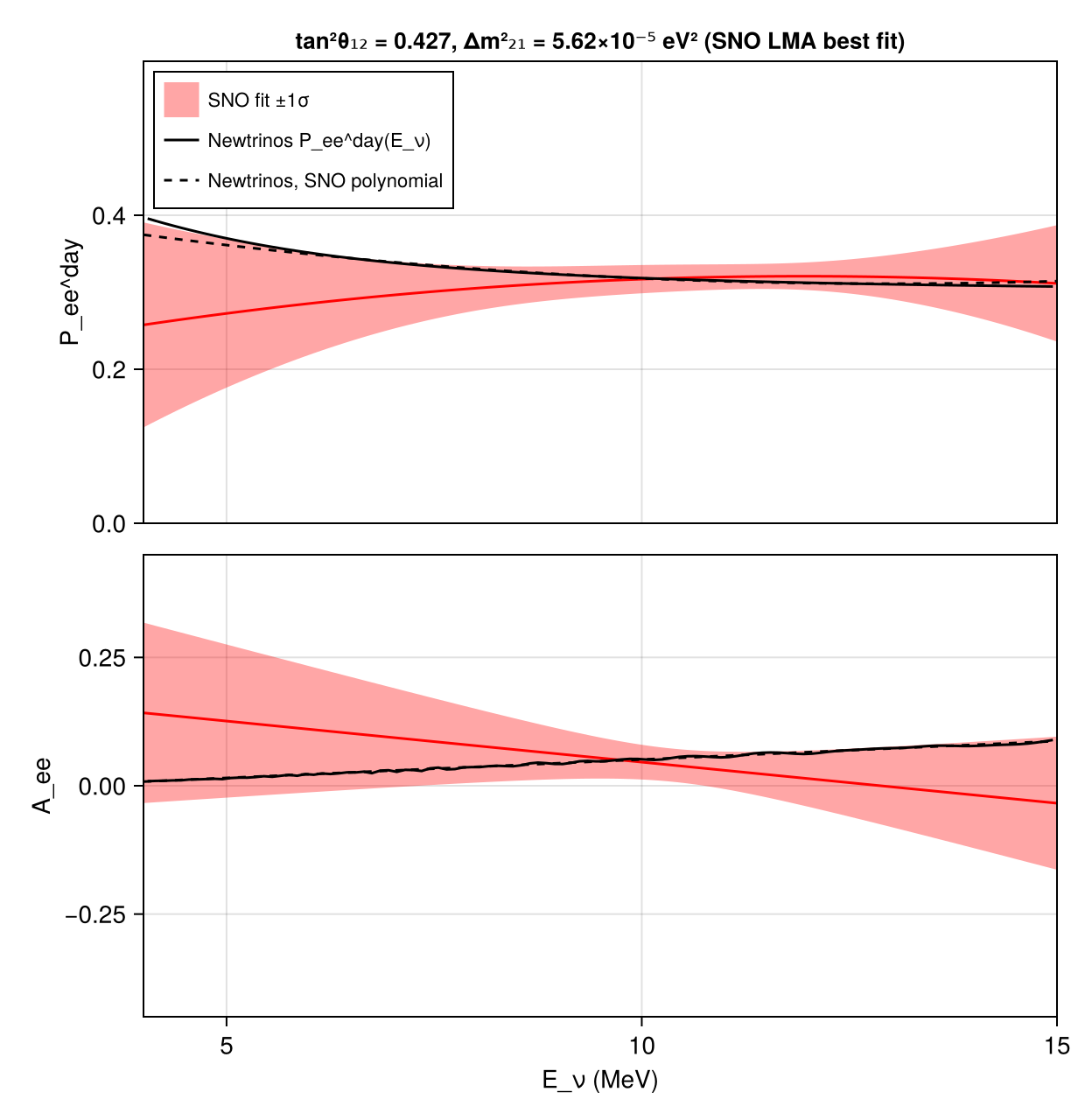
Day-time survival probability and day/night asymmetry vs. E_ν · Fig. 10
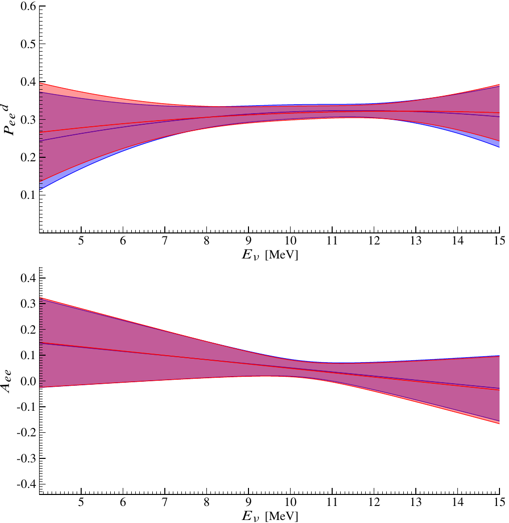
Original figure: SNO, Phys. Rev. C 88, 025501 (2013), Fig. 10, doi:10.1103/PhysRevC.88.025501. Not our work; shown for comparison, all rights with the authors and publisher.
Known limitations
- Below Δm²₂₁ ≈ 10⁻⁷ eV² the conversion of ⁸B neutrinos in the Sun is non-adiabatic; Newtrinos computes it numerically through the solar density profile where Parke's level-crossing estimate is not negligible (an earlier, purely adiabatic version did not close the LOW island). This makes the scan of the low-Δm² region slow (the run takes hours instead of minutes).
- Only the SNO-only two-flavour analysis is reproduced; the panels combining SNO with the other solar experiments and KamLAND (Figs. 15–16) are covered by the global solar entries (Super-Kamiokande IV, NuFIT 6.0).
- The statistical and systematic uncertainties of Table X of the maximum-likelihood fit are symmetrised and added in quadrature; the B23 ⁸B spectrum shape is used at its central value.
- The night-averaged asymmetry of the model (lower panel of Fig. 10, solid black) shows wiggles above 12 MeV from the 20 cos(zenith) night bins of the module's default site; the polynomial projection used in the likelihood (dashed) is smooth.
- Fig. 10 shows SNO's fitted polynomial bands; Newtrinos shows its model prediction at SNO's LMA best fit, together with its own projection onto the polynomials, against SNO's maximum-likelihood band (±1σ from the fitted coefficients and their correlation matrix).
Reproduce
git clone https://github.com/Newtrinos-org/Newtrinos.jl.git && cd Newtrinos.jl && git checkout c6612c255a- Download reproduce.jl into an empty directory.
julia -t 8 --project=/path/to/Newtrinos.jl reproduce.jl
# Reproduction of the SNO combined three-phase analysis, B. Aharmim et al. (SNO), Phys. Rev. C 88, 025501 (2013)
# [arXiv:1109.0763], with the Newtrinos.jl `sno` module: the SNO-only two-flavour (θ₁₂, Δm²₂₁) contour (Fig. 14) and
# the day-time survival probability / day-night asymmetry parameterisation (Fig. 10).
# Run from this directory with the Newtrinos.jl environment at the pinned commit:
#   julia -t 16 --project=<path to Newtrinos.jl> reproduce.jl
using Newtrinos, Distributions, DensityInterface, CairoMakie, CSV, DataFrames, LinearAlgebra, Printf

cd(@__DIR__); mkpath("ours"); mkpath("results")
BLAS.set_num_threads(1)
const SF = Newtrinos.solar_flux

# SNO prescription: two flavours (θ₁₃ = 0), ⁸B flux free; the B23 ⁸B shape at its central value.
# Independent flux normalisations so that the ⁸B flux can be left free.
physics = merge(Newtrinos.solar_common.default_physics(),
                (solar_flux = SF.configure(SF.SolarFluxConfig(systematics = SF.SSMPriors())),))
sno = Newtrinos.sno.configure(physics)
p0 = merge(Newtrinos.get_params((; sno)), (θ₁₃ = 0.0, solar_b8_shape = 0.0))
obs = sno.assets.observed

# −2 ln L as a function of the oscillation parameters, minimised over the ⁸B normalisation. The flux enters only the
# first observable, linearly, so χ² is exactly quadratic in it: three evaluations give the minimum.
χ²(p) = (d = sno.forward_model(p); -2 * (logdensityof(d, obs) - logdensityof(d, mean(d))))   # (o − e)ᵀ C⁻¹ (o − e)
function χ²_min(t2, dm)
    p = merge(p0, (θ₁₂ = atan(sqrt(t2)), Δm²₂₁ = dm))
    f(n) = χ²(merge(p, (solar_norm_b8 = n,)))
    a, b, c = f(0.9), f(1.0), f(1.1)                  # parabola through n = 0.9, 1.0, 1.1
    curv = (a - 2b + c) / 0.01; slope = (c - a) / 0.2
    n̂ = 1.0 - slope / curv
    f(n̂), n̂
end

t2s = 10 .^ range(-2, 0, length = 81)                  # tan²θ₁₂
dms = 10 .^ range(-8, log10(2e-4), length = 81)        # Δm²₂₁ [eV²]
grid = Matrix{Float64}(undef, length(t2s), length(dms)); norm = similar(grid)
Threads.@threads for k in eachindex(grid)
    i, j = Tuple(CartesianIndices(grid)[k])
    grid[i, j], norm[i, j] = χ²_min(t2s[i], dms[j])
end
Δχ² = grid .- minimum(grid)
CSV.write("results/sno_only_2nu.csv", DataFrame(tan2_theta12 = repeat(t2s, outer = length(dms)), dm2_21 = repeat(dms, inner = length(t2s)),
                                                chi2 = vec(grid), dchi2 = vec(Δχ²), b8_flux_1e6 = vec(norm) .* physics.solar_flux.nominal.b8 ./ 1e6))

# best fits in the LMA (Δm² > 1e-5) and LOW (Δm² < 1e-6) regions; 1σ ranges from the profiles within each region
function region(sel)
    g = copy(grid); g[:, .!sel] .= Inf
    i, j = Tuple(argmin(g)); m = g[i, j]
    pt = vec(minimum(g, dims = 2)) .- m; pd = vec(minimum(g, dims = 1)) .- m
    (t2 = t2s[i], dm = dms[j], χ² = m, t2r = extrema(t2s[pt .<= 1]), dmr = extrema(dms[pd .<= 1]))
end
lma = region(dms .> 1e-5); low = region(dms .< 1e-6)
open("results/summary.txt", "w") do io
    for (name, r, ref) in (("LMA", lma, "SNO: tan²θ₁₂ = 0.427 +0.033/−0.029, Δm²₂₁ = 5.62 +1.92/−1.36 e-5 eV², χ²/ndf = 1.39/3"),
                           ("LOW", low, "SNO: tan²θ₁₂ = 0.427 +0.043/−0.035, Δm²₂₁ = 1.35 +0.35/−0.14 e-7 eV², χ²/ndf = 1.41/3"))
        @printf(io, "%s: tan²θ₁₂ = %.3f [%.3f, %.3f], Δm²₂₁ = %.3g [%.3g, %.3g] eV², χ²/ndf = %.2f/3\n     %s\n",
                name, r.t2, r.t2r..., r.dm, r.dmr..., r.χ², ref)
    end
end
print(read("results/summary.txt", String))

# --- Fig. 14: SNO-only two-flavour contour ---
levels = [quantile(Chisq(2), cl) for cl in (0.6827, 0.95, 0.9973)]
fig = Figure(size = (620, 600))
ax = Axis(fig[1, 1], xscale = log10, yscale = log10, xlabel = "tan²θ₁₂", ylabel = "Δm²₂₁ (eV²)", title = "Newtrinos: SNO only (2ν)")
for (l, c, w, lab) in zip(levels, (:lightgreen, :green, :darkgreen), (2, 3, 2), ("68.27 % C.L.", "95.00 % C.L.", "99.73 % C.L."))
    contour!(ax, t2s, dms, Δχ², levels = [l], color = c, linewidth = w, label = lab)
end
scatter!(ax, [lma.χ² <= low.χ² ? lma.t2 : low.t2], [lma.χ² <= low.χ² ? lma.dm : low.dm], color = :green, label = "Minimum")
scatter!(ax, [0.427, 0.427], [5.62e-5, 1.35e-7], marker = :xcross, color = :black, label = "SNO best fits")
xlims!(ax, 1e-2, 1); ylims!(ax, 1e-8, 2e-4)
axislegend(ax, position = :lt)
save("ours/fig_sno_only_2nu.png", fig)

# --- Fig. 10: P_ee^day and A_ee, SNO's parameterisation (±1σ band from the covariance) vs. Newtrinos at SNO's LMA best fit ---
pb = merge(p0, (θ₁₂ = atan(sqrt(0.427)), Δm²₂₁ = 5.62e-5))
Pd, Pn = Newtrinos.sno.day_night_prob(pb, sno.physics, sno.assets)
θfit = Newtrinos.sno.fit_polynomials(Pd, Pn, sno.assets)
C = Matrix(sno.assets.cov)
E = range(4, 15, length = 221); x = E .- 10
Pobs = obs[2] .+ obs[3] .* x .+ obs[4] .* x .^ 2
σP = [sqrt([1, t, t^2]' * C[2:4, 2:4] * [1, t, t^2]) for t in x]
Aobs = obs[5] .+ obs[6] .* x
σA = [sqrt([1, t]' * C[5:6, 5:6] * [1, t]) for t in x]
CSV.write("results/coefficients.csv", DataFrame(coefficient = ["c0", "c1", "c2", "a0", "a1"], sno_measured = obs[2:6],
                                                sno_sigma = sqrt.(diag(C))[2:6], newtrinos_at_sno_lma_best_fit = θfit))
fig = Figure(size = (620, 640))
ax = Axis(fig[1, 1], ylabel = "P_ee^day", title = "tan²θ₁₂ = 0.427, Δm²₂₁ = 5.62×10⁻⁵ eV² (SNO LMA best fit)", titlesize = 13)
band!(ax, E, Pobs .- σP, Pobs .+ σP, color = (:red, 0.35), label = "SNO fit ±1σ")
lines!(ax, E, Pobs, color = :red)
Em = sno.assets.E; sel = 4 .<= Em .<= 15
lines!(ax, Em[sel], Pd[sel], color = :black, label = "Newtrinos P_ee^day(E_ν)")
lines!(ax, E, θfit[1] .+ θfit[2] .* x .+ θfit[3] .* x .^ 2, color = :black, linestyle = :dash, label = "Newtrinos, SNO polynomial")
xlims!(ax, 4, 15); ylims!(ax, 0, 0.6); axislegend(ax, position = :lt, labelsize = 11); hidexdecorations!(ax, grid = false)
ax2 = Axis(fig[2, 1], xlabel = "E_ν (MeV)", ylabel = "A_ee")
band!(ax2, E, Aobs .- σA, Aobs .+ σA, color = (:red, 0.35)); lines!(ax2, E, Aobs, color = :red)
lines!(ax2, Em[sel], (2 .* (Pn .- Pd) ./ (Pn .+ Pd))[sel], color = :black)
lines!(ax2, E, θfit[4] .+ θfit[5] .* x, color = :black, linestyle = :dash)
xlims!(ax2, 4, 15); ylims!(ax2, -0.45, 0.45)
save("ours/fig_pee_day_asym.png", fig)
Provenance
| Newtrinos.jl commit | c6612c255a (sno, solar_flux, solar_common, osc, earth_layers) |
|---|---|
| Run date | 2026-10-21T18:36:18Z |
| Wall time | 358.7 min (128 threads) |
| Julia | 1.12.5 |
| Machine | AMD EPYC 7702P 64-Core Processor, 128 hardware threads, Linux |
| Environment | newtrinos_Manifest.toml · run.toml |
Downloads
CSV files hold one row per scan point: the scanned and profiled parameters
(sin2_theta23, dm2_32 in eV², dcp in rad, nuisance parameters), dchi2 = −2Δ log L
and the log-likelihood. JLD2 files contain the full NewtrinosResult objects.
| File | Size | SHA-256 |
|---|---|---|
| ours/fig_pee_day_asym.png | 107.0 kB | db06829c9ba2… |
| ours/fig_sno_only_2nu.png | 92.7 kB | 18d68956e50a… |
| results/coefficients.csv | 322 B | e49cd08165c4… |
| results/sno_only_2nu.csv | 615.3 kB | 467fd2b485f0… |
| results/summary.txt | 441 B | 4d68ad201362… |