
Borexino · Phys. Rev. D 100, 082004 (2019)
First Simultaneous Precision Spectroscopy of pp, ⁷Be, and pep Solar Neutrinos with Borexino Phase-II
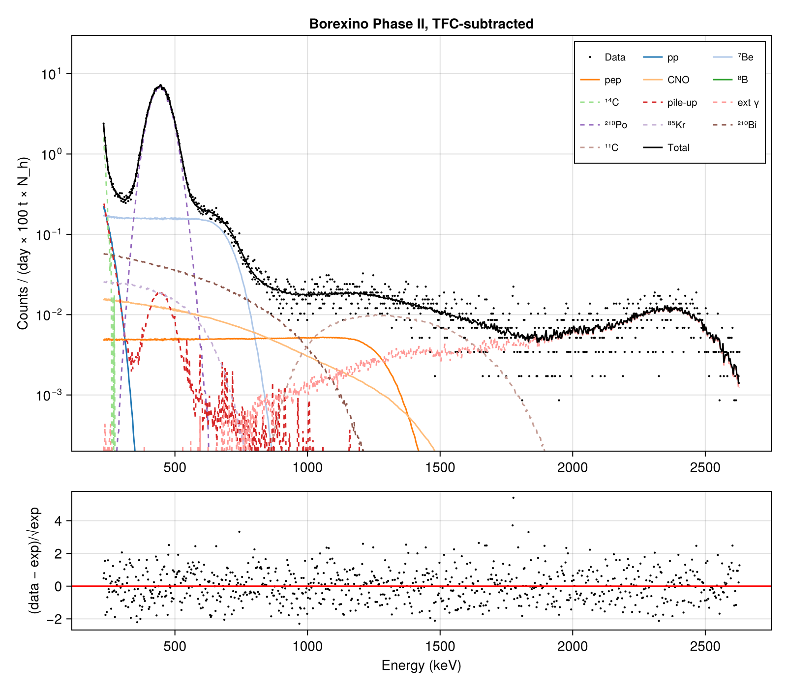
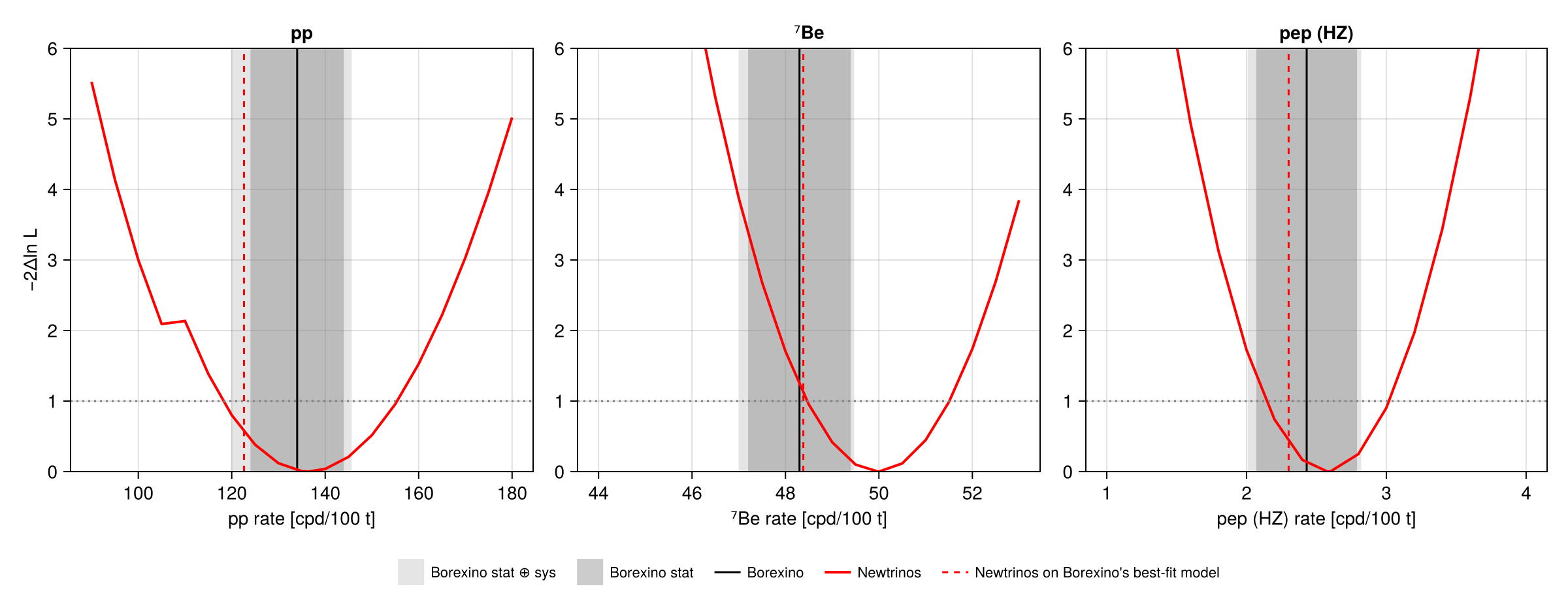
Interaction rates of pp, ⁷Be and pep solar neutrinos from the Borexino Phase-II TFC-subtracted energy spectrum (N_h estimator, open data of Nature 562, 505 (2018) Fig. 2a), fitted from 231 keV with the Newtrinos module borexino_ph2_spectrum: solar components from the Borexino MC shapes with an energy response calibrated on Borexino's best-fit spectrum and rates predicted by Newtrinos (here freed individually), backgrounds from Borexino's own fitted components (extracted from the vector graphics of Fig. 6a) with free normalisations, CNO constrained to the HZ-SSM value 4.92 ± 0.56 cpd/100 t, ¹⁴C (±5 %) and pile-up (±2 %) constrained as in Borexino's MC fit. Newtrinos finds pp = 136 [118, 155], ⁷Be = 50.0 [48.5, 51.5], pep = 2.58 [2.15, 3.02] cpd/100 t (Borexino: 134 ± 10 +6/−10, 48.3 ± 1.1 +0.4/−0.7, 2.43 ± 0.36 +0.15/−0.22), with 884 for 851 bins (Poisson deviance).
Figures
TFC-subtracted spectrum with the fit components · Fig. 6a
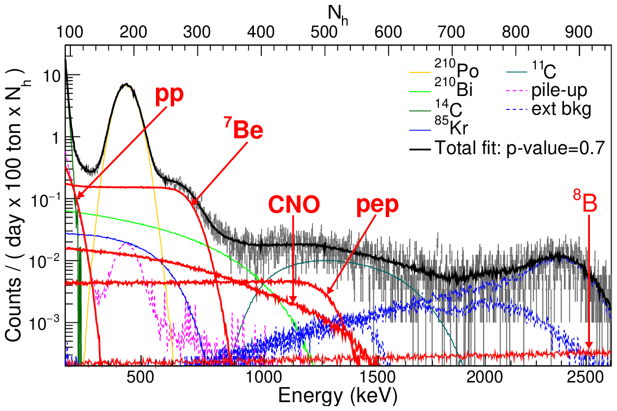
Original figure: Borexino, Phys. Rev. D 100, 082004 (2019), Fig. 6a, doi:10.1103/PhysRevD.100.082004. Not our work; shown for comparison, all rights with the authors and publisher.
Profiles of the pp, ⁷Be and pep interaction rates vs. Borexino's results · Table (results)
Table (results)
Known limitations
- Borexino's fit is multivariate (energy, radial and pulse-shape distributions, TFC-subtracted and TFC-tagged spectra); only the TFC-subtracted energy spectrum is public and used here. Newtrinos' intervals (−2Δln L = 1, statistical plus the module's nuisances) are therefore wider for pp than Borexino's statistical error.
- Closure test: fitting Borexino's own best-fit model of the spectrum, Newtrinos returns pp = 122.6, ⁷Be = 48.4 and pep = 2.30 cpd/100 t instead of 134, 48.3 and 2.43. The −9 % for pp comes from the solar MC shapes of the open data (Phase-III, in keV) mapped linearly onto the Phase-II N_h scale, which is least accurate at the 230–270 keV threshold where the pp signal lies.
- The background shapes are Borexino's fitted components at Borexino's best-fit detector response (with free normalisations); the bin-to-bin structure of the discrete N_h estimator under the ²¹⁰Po peak, present in the data and in Borexino's total fit but not in the drawn smooth curves, is recovered as (total − Σ components) and added to the ²¹⁰Po shape.
- Each solar component has the shape of its MC spectrum; only its rate follows the oscillation parameters (the energy dependence of P_ee within the pp and CNO spectra is not applied).
- The rates are interaction rates without the Borexino detection efficiency corrections being refitted; the first 8 bins (N_h 92–99, 212–229 keV), where Borexino's own fit deviates strongly from the data, are excluded.
Reproduce
git clone https://github.com/Newtrinos-org/Newtrinos.jl.git && cd Newtrinos.jl && git checkout c6612c255a- Download reproduce.jl into an empty directory.
julia -t 8 --project=/path/to/Newtrinos.jl reproduce.jl
# Reproduction of Borexino, Phys. Rev. D 100, 082004 (2019) [arXiv:1707.09279]: pp, ⁷Be and pep interaction rates from
# the Phase-II TFC-subtracted spectrum (Fig. 6a, MC-method fit) with the Newtrinos module borexino_ph2_spectrum.
# Run from this directory with the Newtrinos.jl environment at the pinned commit:
#   julia -t 16 --project=<path to Newtrinos.jl> reproduce.jl
using Newtrinos, Distributions, DensityInterface, Optim, ADTypes, ForwardDiff, CairoMakie, Printf, CSV, DataFrames

cd(@__DIR__); mkpath("ours"); mkpath("results")
const B = Newtrinos.borexino_ph2_spectrum
# independent flux normalisations, so that pp, ⁷Be, pep and CNO can be freed individually
physics = merge(B.default_physics(), (solar_flux = Newtrinos.solar_flux.configure(
    Newtrinos.solar_flux.SolarFluxConfig(systematics = Newtrinos.solar_flux.SSMPriors())),))
bx = B.configure(physics)
exps = (borexino_ph2_spectrum = bx,)
llh = Newtrinos.generate_likelihood(exps)
p0 = Newtrinos.get_params(exps)
priors = Newtrinos.get_priors(exps)

# Borexino conditions (HZ): pp, ⁷Be, pep free; CNO constrained to 4.92 ± 0.56 cpd/100 t (¹³N, ¹⁵O, ¹⁷F share one
# normalisation); ⁸B, hep and the oscillation parameters at the Newtrinos defaults; backgrounds and energy response
# profiled with the module priors (¹⁴C ±5 %, pile-up ±2 %).
rate0 = B.solar_rates(p0, bx.physics, bx.assets)            # rates [cpd/100 t] at unit normalisations
nuis = collect(keys(bx.params))
toparams(x) = merge(p0, (solar_norm_pp = x[1], solar_norm_be7 = x[2], solar_norm_pep = x[3],
                         solar_norm_n13 = x[4], solar_norm_o15 = x[4], solar_norm_f17 = x[4]),
                    NamedTuple{Tuple(nuis)}(Tuple(x[5:end])))
cno_prior = Normal(4.92, 0.56)
nlp(x) = -(logdensityof(llh, toparams(x)) + logpdf(cno_prior, x[4] * rate0.cno) +
           sum(logpdf(priors[k], x[4+i]) for (i, k) in enumerate(nuis)))
lo = vcat(0.2, 0.5, 0.0, 0.0, [minimum(priors[k]) for k in nuis]); hi = vcat(2.0, 1.5, 3.0, 3.0, [maximum(priors[k]) for k in nuis])
x0 = vcat(1.0, 1.0, 1.0, 4.92 / rate0.cno, [p0[k] for k in nuis])
function minimise(f, x0, lo, hi)
    r = optimize(f, lo, hi, clamp.(x0, lo .+ 1e-6, hi .- 1e-6), Fminbox(LBFGS()),
                 Optim.Options(iterations=1000, outer_iterations=10, g_tol=1e-6); autodiff=ADTypes.AutoForwardDiff())
    Optim.minimizer(r), Optim.minimum(r)
end
xb, mb = minimise(nlp, x0, lo, hi)
pb = toparams(xb)
best = B.solar_rates(pb, bx.physics, bx.assets)

# profiles of the pp, ⁷Be and pep rates (−2Δln L, all other parameters profiled)
grids = (pp = collect(90.0:5.0:180.0), be7 = collect(44.0:0.5:53.0), pep = collect(1.0:0.2:4.0))
# each profile is computed outwards from the best fit, starting every point from its neighbour's solution and from the
# global best fit (the better of the two is kept), to avoid local minima; the three rates run in parallel
profiles = Dict{Symbol, Vector{Float64}}()
lk = ReentrantLock()
Threads.@threads for (i, k) in collect(enumerate((:pp, :be7, :pep)))
    g = grids[k]; prof = zeros(length(g))
    keep = setdiff(eachindex(xb), i)
    ib = searchsortedfirst(g, best[k])
    for order in (ib:length(g), reverse(1:ib-1))
        ystart = xb[keep]
        for j in order
            fix(y) = (x = Vector{eltype(y)}(undef, length(xb)); x[keep] = y; x[i] = g[j] / rate0[k]; x)
            r1 = minimise(y -> nlp(fix(y)), ystart, lo[keep], hi[keep])
            r2 = minimise(y -> nlp(fix(y)), xb[keep], lo[keep], hi[keep])
            y, m = r1[2] <= r2[2] ? r1 : r2
            prof[j] = 2 * (m - mb); ystart = y
        end
    end
    lock(lk) do
        profiles[k] = prof
    end
    CSV.write("results/profile_$(k).csv", DataFrame(rate_cpd100t = g, minus2_dlnL = prof))
end
# 68 % interval from −2Δln L = 1 (linear interpolation, best fit included)
function interval(k)
    g = vcat(grids[k], best[k]); p = vcat(profiles[k], 0.0); o = sortperm(g); g, p = g[o], p[o]
    ib = findfirst(==(0.0), p)
    cross(i1, i2) = g[i1] + (1 - p[i1]) * (g[i2] - g[i1]) / (p[i2] - p[i1])
    il = findlast(>(1), p[1:ib]); iu = ib - 1 + findfirst(>(1), p[ib:end])
    (il === nothing ? NaN : cross(il, il + 1)), (iu === nothing ? NaN : cross(iu - 1, iu))
end

# closure test: the same fit applied to Borexino's own best-fit model (Fig. 2a data − residual × error)
target = bx.assets.spectrum.bestfit
nlp_bf(x) = (μ = max.(B.get_expected(toparams(x), bx.physics, bx.assets).total, 1e-9);
             sum(μ .- target .* log.(μ)) - logpdf(cno_prior, x[4] * rate0.cno) - sum(logpdf(priors[k], x[4+i]) for (i, k) in enumerate(nuis)))
xc, _ = minimise(nlp_bf, xb, lo, hi)
closure = B.solar_rates(toparams(xc), bx.physics, bx.assets)

paper = (pp = (134.0, 10.0, 6.0, 10.0), be7 = (48.3, 1.1, 0.4, 0.7), pep = (2.43, 0.36, 0.15, 0.22))   # value, stat, +sys, −sys
ex = B.get_expected(pb, bx.physics, bx.assets)
N = bx.assets.observed
deviance = 2 * sum(ex.total .- N .+ N .* log.(max.(N, 1e-300) ./ ex.total))
open("results/summary.txt", "w") do io
    @printf(io, "best fit (deviance %.1f for %d bins): ", deviance, length(N))
    println(io, join([@sprintf("%s = %.2f [%.2f, %.2f]", k, best[k], interval(k)...) for k in (:pp, :be7, :pep)], ", "),
            @sprintf(", CNO = %.2f cpd/100 t", best.cno))
    println(io, "closure (fit to Borexino's best-fit model): ", join([@sprintf("%s = %.2f", k, closure[k]) for k in (:pp, :be7, :pep)], ", "))
    println(io, "Borexino (PRD 100, 082004, HZ): ", join([@sprintf("%s = %.2f ± %.2f (stat) +%.2f/−%.2f (sys)", k, paper[k]...) for k in (:pp, :be7, :pep)], ", "))
    println(io, "nuisances: ", join([@sprintf("%s=%.3g", replace(string(k), "borexino_ph2s_" => ""), v) for (k, v) in zip(nuis, xb[5:end])], " "))
end
print(read("results/summary.txt", String))

# Fig. 6a: spectrum and components at the best fit
save("ours/fig6a_spectrum.png", bx.plot(pb))

# rate profiles vs. Borexino's results
fig = Figure(size = (1200, 470))
for (i, (k, lab)) in enumerate(((:pp, "pp"), (:be7, "⁷Be"), (:pep, "pep (HZ)")))
    ax = Axis(fig[1, i], xlabel = "$lab rate [cpd/100 t]", ylabel = i == 1 ? "−2Δln L" : "", title = lab)
    v, st, sp, sm = paper[k]
    vspan!(ax, [v - sqrt(st^2 + sm^2)], [v + sqrt(st^2 + sp^2)], color = (:gray, 0.2), label = "Borexino stat ⊕ sys")
    vspan!(ax, [v - st], [v + st], color = (:gray, 0.4), label = "Borexino stat")
    vlines!(ax, [v], color = :black, label = "Borexino")
    g = vcat(grids[k], best[k]); p = vcat(profiles[k], 0.0); o = sortperm(g)
    lines!(ax, g[o], p[o], color = :red, linewidth = 2, label = "Newtrinos")
    vlines!(ax, [closure[k]], color = :red, linestyle = :dash, label = "Newtrinos on Borexino's best-fit model")
    hlines!(ax, [1.0], color = :gray, linestyle = :dot)
    ylims!(ax, 0, 6)
    i == 1 && Legend(fig[2, 1:3], ax, orientation = :horizontal, framevisible = false, labelsize = 11)
end
save("ours/rate_profiles.png", fig)
Provenance
| Newtrinos.jl commit | c6612c255a (solar_flux, solar_xsec, solar_common, borexino_ph2_spectrum) |
|---|---|
| Run date | 2026-10-21T16:58:00Z |
| Wall time | 5.2 min (128 threads) |
| Julia | 1.12.5 |
| Machine | AMD EPYC 7702P 64-Core Processor, 128 hardware threads, Linux |
| Environment | newtrinos_Manifest.toml · run.toml |
Downloads
CSV files hold one row per scan point: the scanned and profiled parameters
(sin2_theta23, dm2_32 in eV², dcp in rad, nuisance parameters), dchi2 = −2Δ log L
and the log-likelihood. JLD2 files contain the full NewtrinosResult objects.
| File | Size | SHA-256 |
|---|---|---|
| ours/fig6a_spectrum.png | 367.0 kB | da7685ddf2fe… |
| ours/rate_profiles.png | 154.9 kB | 596e4112e847… |
| results/profile_be7.csv | 484 B | 405575fe02c4… |
| results/profile_pep.csv | 390 B | 9c2dc59c68e8… |
| results/profile_pp.csv | 492 B | 69e77af38d41… |
| results/summary.txt | 538 B | aaf435f429b5… |