
COHERENT Collaboration · Phys. Rev. D 106, 032003 (2022)
Simulating the neutrino flux from the Spallation Neutron Source for the COHERENT experiment
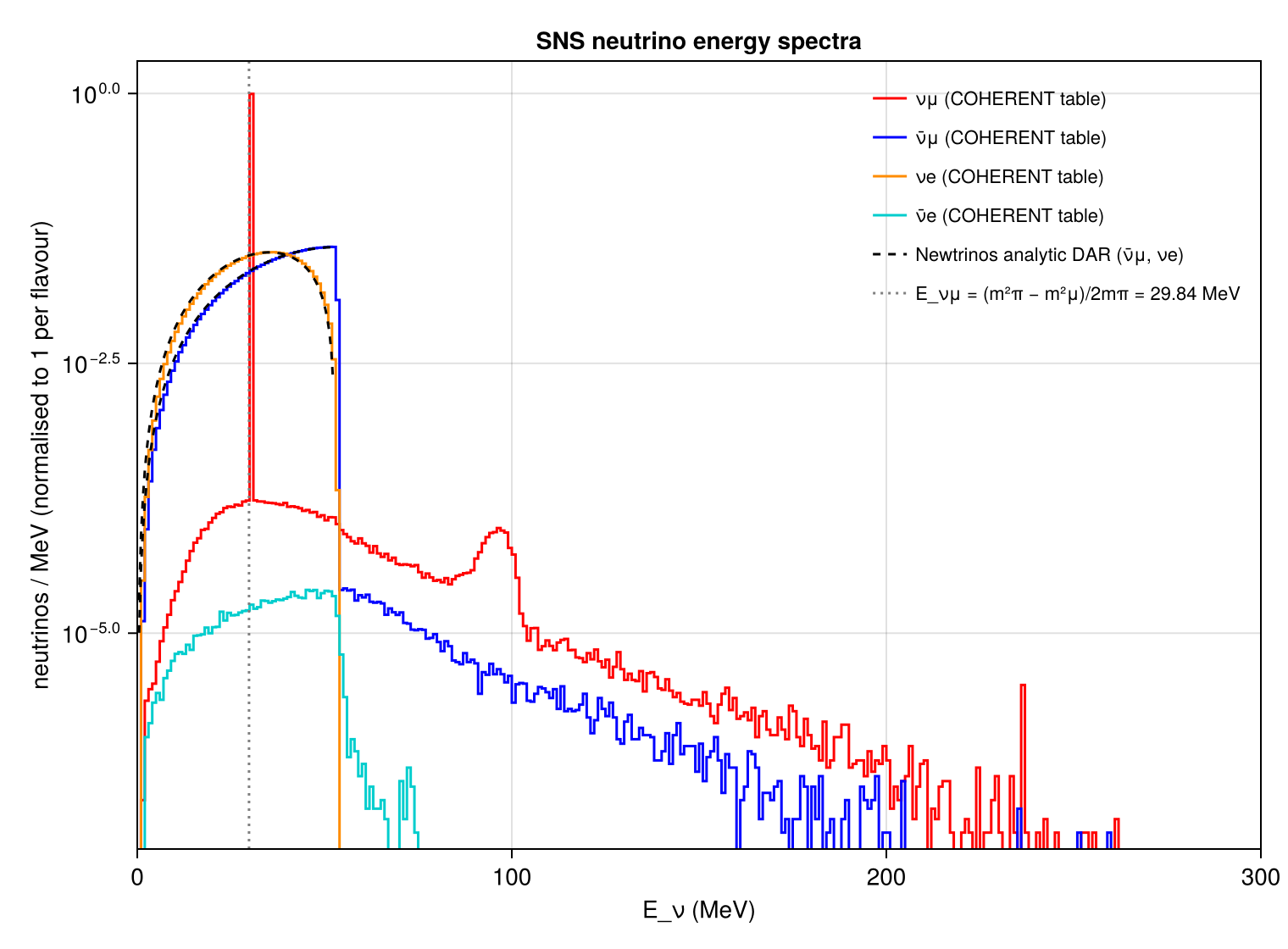
The SNS pion-decay-at-rest flux of Newtrinos.jl (module sns_flux): the energy–time tables of the COHERENT Geant4 simulation (shipped with the CsI data release and used by the COHERENT modules) and the analytic decay-at-rest spectra, compared with the paper's energy and timing distributions, its flavour yields, and the decay kinematics (29.79 MeV prompt line, mμ/2 endpoint, muon lifetime).
Figures
Neutrino energy spectra · Fig. 13 (top)
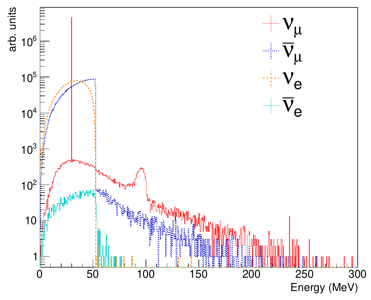
Original figure: COHERENT Collaboration, Phys. Rev. D 106, 032003 (2022), Fig. 13 (top), doi:10.1103/PhysRevD.106.032003. Not our work; shown for comparison, all rights with the authors and publisher.
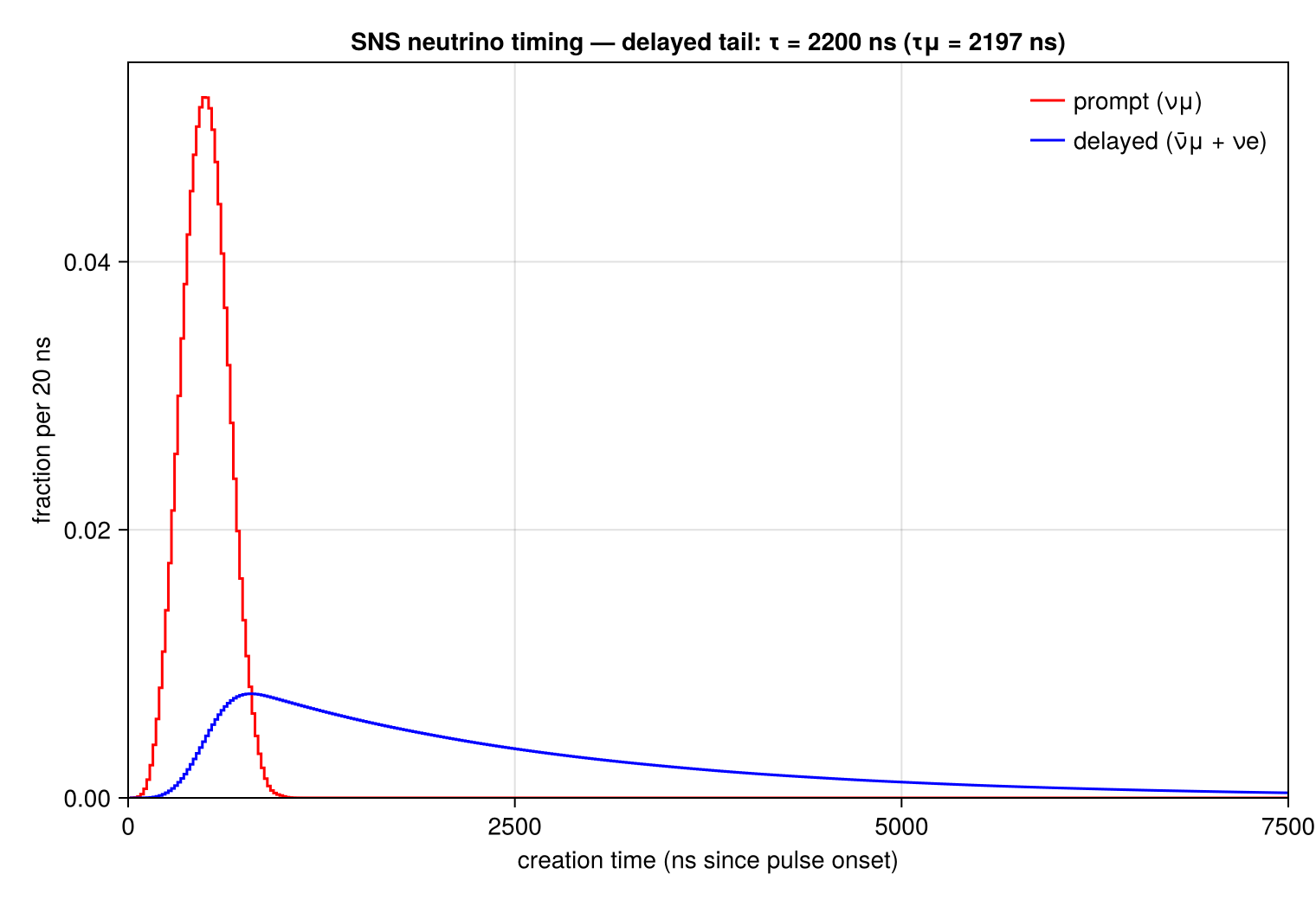
Neutrino creation-time distributions · Fig. 13 (bottom)
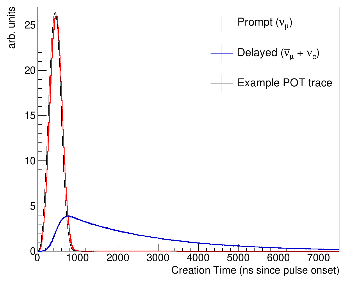
Original figure: COHERENT Collaboration, Phys. Rev. D 106, 032003 (2022), Fig. 13 (bottom), doi:10.1103/PhysRevD.106.032003. Not our work; shown for comparison, all rights with the authors and publisher.
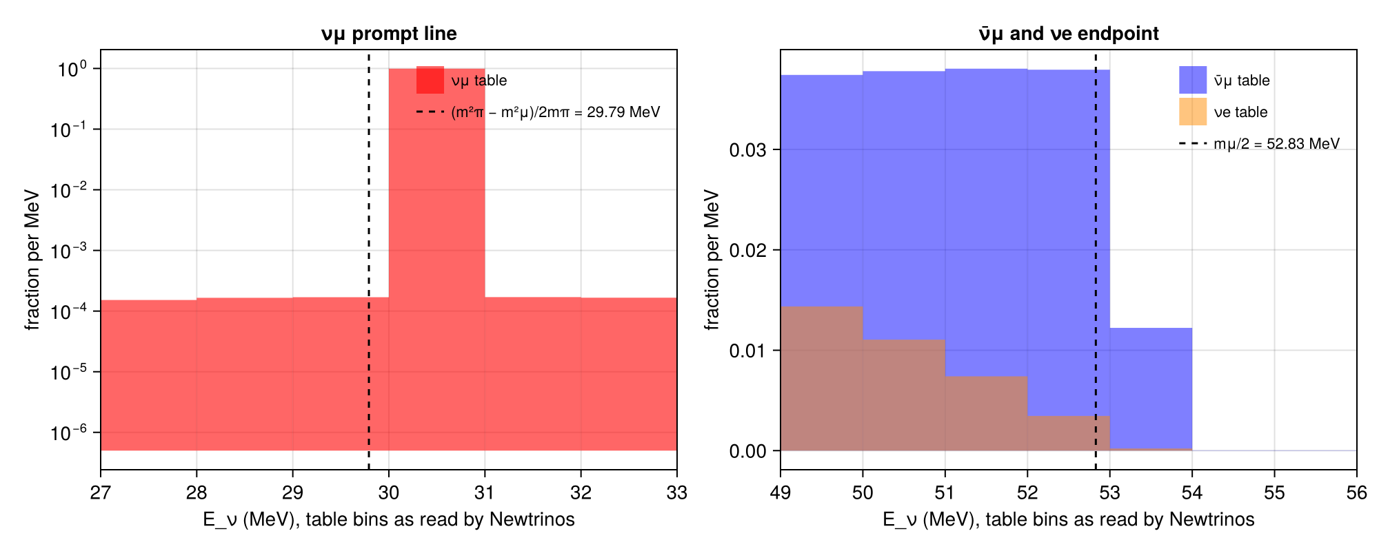
Prompt line and Michel endpoint in the flux tables, at the energies Newtrinos assigns · not in the paper
not in the paper
Known limitations
- Energy offset: COHERENT's flux histogram (snsFlux2D.root, and the CSV tables derived from it) has the 29.79 MeV prompt νμ line in its [30, 31] MeV bin and the Michel spectra extending one third of a bin past mμ/2 = 52.83 MeV, i.e. the histogram was filled with energies rounded to the nearest MeV. Newtrinos reads the bin centres (n + 0.5 MeV), so all SNS flux energies used in the COHERENT modules are about 0.5 MeV too high (ν̄μ endpoint 53.32 MeV, prompt line 30.5 MeV). For a cross section rising like E², this raises the predicted CEvNS rate by an estimated few percent; not yet propagated to the COHERENT entries.
- Flavour yields, the prompt-line fraction (99.2 % vs. the paper's 98.9 % from π⁺ DAR), the shapes of the decay-in-flight tails and the timing agree with the paper; the delayed component decays with τ = 2200 ns (τμ = 2197 ns).
- The analytic mode uses mμ = 105.6 MeV (prompt line 29.84 MeV instead of 29.79 MeV) and a default 0.09 ν per POT per flavour (paper: 0.0875 at 1 GeV, within the 10 % prior).
- The tables are the ones of the CsI 2020 release; the paper's Fig. 13 shows the same simulation in finer energy bins.
Reproduce
git clone https://github.com/Newtrinos-org/Newtrinos.jl.git && cd Newtrinos.jl && git checkout de27463fde- Download reproduce.jl into an empty directory.
julia -t 8 --project=/path/to/Newtrinos.jl reproduce.jl
# The SNS neutrino flux in Newtrinos.jl (module `sns_flux`) compared with COHERENT, "Simulating the neutrino flux
# from the Spallation Neutron Source for the COHERENT experiment", Phys. Rev. D 106, 032003 (2022), Fig. 13.
# Run from this directory with the Newtrinos.jl environment at the pinned commit:
#   julia --project=<path to Newtrinos.jl> reproduce.jl
using Newtrinos, CairoMakie, CSV, DataFrames, Printf, Statistics

cd(@__DIR__); mkpath("ours"); mkpath("results")

# data mode: the COHERENT energy-time flux tables (Geant4 SNS simulation, 1 ns × 1 MeV) shipped with the CsI release
tb = collect(0.0:20.0:15000.0)
data = Newtrinos.sns_flux.configure(exposure = 1.0, distance = 19.3, ecut = 600.0, tcut = 15000.0, tbins = tb)
ad = data.assets
E = ad.E
spec(f) = vec(sum(f, dims = 2))            # energy spectrum (summed over time)
tdist(f) = vec(sum(f, dims = 1))           # time distribution (summed over energy)
D = (νμ = ad.flux_mu, ν̄μ = ad.flux_mu_bar, νe = ad.flux_e, ν̄e = ad.flux_e_bar)
tot = Dict(k => sum(v) for (k, v) in pairs(D))

# analytic mode: pion and muon decay at rest (monoenergetic νμ, Michel spectra for νe and ν̄μ)
ana = Newtrinos.sns_flux.configure(exposure = 1.0, distance = 19.3, use_data = false, E_bin_width = 0.5)
aa = ana.assets

# ---- Fig. 13 (top): energy spectra; tables in 1 MeV bins, analytic spectra scaled to the same per-MeV normalisation
fig = Figure(size = (760, 560))
ax = Axis(fig[1, 1], yscale = log10, xlabel = "E_ν (MeV)", ylabel = "neutrinos / MeV (normalised to 1 per flavour)",
          title = "SNS neutrino energy spectra", limits = (0, 300, 1e-7, 2))
col = (νμ = :red, ν̄μ = :blue, νe = :darkorange, ν̄e = :cyan3)
for k in (:νμ, :ν̄μ, :νe, :ν̄e)
    s = spec(D[k]) ./ tot[:νμ]                 # common normalisation: the νμ total
    stairs!(ax, E, max.(s, 1e-9), step = :center, color = col[k], label = "$k (COHERENT table)")
end
for (k, f) in ((:ν̄μ, aa.flux_mu_bar), (:νe, aa.flux_e))
    lines!(ax, aa.E, f ./ sum(f) .* 2 .* (tot[k] / tot[:νμ]), color = :black, linestyle = :dash,   # 0.5 MeV → per MeV
           label = k == :ν̄μ ? "Newtrinos analytic DAR (ν̄μ, νe)" : nothing)
end
vlines!(ax, [Newtrinos.sns_flux.ep], color = :gray, linestyle = :dot, label = "E_νμ = (m²π − m²μ)/2mπ = $(round(Newtrinos.sns_flux.ep, digits = 2)) MeV")
axislegend(ax, position = :rt, framevisible = false, labelsize = 11)
save("ours/fig13a_energy.png", fig)

# ---- Fig. 13 (bottom): creation-time distributions, prompt (νμ) and delayed (ν̄μ + νe)
tc = (tb[1:end-1] .+ tb[2:end]) ./ 2
prompt, delayed = tdist(D[:νμ]), tdist(D[:ν̄μ]) .+ tdist(D[:νe])
# lifetime of the delayed component from an exponential fit to its tail (t > 2 µs, after the proton pulse)
sel = (tc .> 2000) .& (tc .< 12000) .& (delayed .> 0)
x, y = tc[sel], log.(delayed[sel])
slope = sum((x .- mean(x)) .* (y .- mean(y))) / sum((x .- mean(x)) .^ 2)
τ = -1 / slope
fig = Figure(size = (760, 520))
ax = Axis(fig[1, 1], xlabel = "creation time (ns since pulse onset)", ylabel = "fraction per 20 ns",
          title = @sprintf("SNS neutrino timing — delayed tail: τ = %.0f ns (τμ = 2197 ns)", τ), limits = (0, 7500, 0, nothing))
stairs!(ax, tc, prompt ./ sum(prompt), step = :center, color = :red, label = "prompt (νμ)")
stairs!(ax, tc, delayed ./ sum(delayed), step = :center, color = :blue, label = "delayed (ν̄μ + νe)")
axislegend(ax, position = :rt, framevisible = false)
save("ours/fig13b_time.png", fig)

# ---- numbers: flavour fractions, prompt line, endpoint, delayed-tail lifetime, mean energies
const mμ, mπ = 105.6584, 139.5704                         # PDG masses [MeV]
Eline, Eend = (mπ^2 - mμ^2) / (2mπ), mμ / 2                # 29.79 MeV νμ line; 52.83 MeV Michel endpoint
mean_E(k) = sum(E .* spec(D[k])) / tot[k]
michel_mean(f) = sum(aa.E .* f) / sum(f)
sμ = spec(D[:νμ]) ./ tot[:νμ]
iline = argmax(sμ)
# ν̄μ endpoint as seen by Newtrinos: the bin centre where the flat top of the Michel spectrum ends, plus the
# filled fraction of the last (partially filled) bin
sb = spec(D[:ν̄μ]); plateau = maximum(sb)
ilast = findlast(>(0.05plateau), sb)
end_newtrinos = E[ilast] - 0.5 + sb[ilast] / plateau        # lower edge + fill fraction (1 MeV bins)
rows = [
  (quantity = "ν̄μ / νμ (table totals)", newtrinos = tot[:ν̄μ] / tot[:νμ], reference = 0.0875 / 0.0875, note = "paper Table III: 0.0875 / 0.0875 ν per POT"),
  (quantity = "νe / νμ (table totals)", newtrinos = tot[:νe] / tot[:νμ], reference = 0.0872 / 0.0875, note = "paper Table III: 0.0872 / 0.0875"),
  (quantity = "ν̄e / νμ (table totals)", newtrinos = tot[:ν̄e] / tot[:νμ], reference = NaN, note = "small ν̄e component (μ⁻ decay)"),
  (quantity = "νμ fraction in the prompt-line bin", newtrinos = sμ[iline], reference = 0.9894, note = "paper Table III: 98.94 % of νμ from π⁺ DAR"),
  (quantity = "prompt-line energy as used by Newtrinos [MeV]", newtrinos = E[iline], reference = Eline, note = "(m²π − m²μ)/2mπ; table bin [30, 31] MeV"),
  (quantity = "ν̄μ endpoint as used by Newtrinos [MeV]", newtrinos = end_newtrinos, reference = Eend, note = "mμ/2"),
  (quantity = "analytic-mode prompt line [MeV]", newtrinos = Newtrinos.sns_flux.ep, reference = Eline, note = "sns_flux uses mμ = 105.6 MeV"),
  (quantity = "mean E(νe) [MeV], table", newtrinos = mean_E(:νe), reference = michel_mean(aa.flux_e), note = "reference: analytic Michel spectrum (DAR only)"),
  (quantity = "mean E(ν̄μ) [MeV], table", newtrinos = mean_E(:ν̄μ), reference = michel_mean(aa.flux_mu_bar), note = "reference: analytic Michel spectrum (DAR only)"),
  (quantity = "delayed-tail lifetime [ns]", newtrinos = τ, reference = 2196.98, note = "muon lifetime (PDG)"),
  (quantity = "analytic default ν per POT per flavour", newtrinos = ana.params.sns_nu_per_POT, reference = 0.0875, note = "paper: 0.0875 (QGSP_BERT, 1 GeV); prior 0.09 ± 0.009"),
]

# zoom on the prompt line and the Michel endpoint: table bins at the energies Newtrinos assigns to them
fig = Figure(size = (1000, 400))
for (k, (lo, hi, ttl)) in enumerate(((27, 33, "νμ prompt line"), (49, 56, "ν̄μ and νe endpoint")))
    local ax = Axis(fig[1, k], title = ttl, xlabel = "E_ν (MeV), table bins as read by Newtrinos", ylabel = "fraction per MeV",
                    yscale = k == 1 ? log10 : identity, limits = (lo, hi, nothing, nothing))
    if k == 1
        barplot!(ax, E, max.(sμ, 1e-6), width = 1.0, gap = 0, color = (:red, 0.6), label = "νμ table")
        vlines!(ax, [Eline], color = :black, linestyle = :dash, label = "(m²π − m²μ)/2mπ = 29.79 MeV")
    else
        barplot!(ax, E, sb ./ sum(sb), width = 1.0, gap = 0, color = (:blue, 0.5), label = "ν̄μ table")
        barplot!(ax, E, spec(D[:νe]) ./ tot[:νe], width = 1.0, gap = 0, color = (:darkorange, 0.5), label = "νe table")
        vlines!(ax, [Eend], color = :black, linestyle = :dash, label = "mμ/2 = 52.83 MeV")
    end
    axislegend(ax, position = :rt, framevisible = false, labelsize = 11)
end
save("ours/energy_offset.png", fig)
tab = DataFrame(rows)
CSV.write("results/sns_flux_checks.csv", tab)
CSV.write("results/sns_flux_energy_spectra.csv",
          DataFrame(E_MeV = E, numu = spec(D[:νμ]) ./ tot[:νμ], numubar = spec(D[:ν̄μ]) ./ tot[:νμ],
                    nue = spec(D[:νe]) ./ tot[:νμ], nuebar = spec(D[:ν̄e]) ./ tot[:νμ]))
show(stdout, tab, allrows = true, truncate = 60); println()
Provenance
| Newtrinos.jl commit | de27463fde (sns_flux) |
|---|---|
| Run date | 2026-10-05T07:43:21Z |
| Wall time | 1.5 min (2 threads) |
| Julia | 1.13.0 |
| Machine | 13th Gen Intel(R) Core(TM) i7-13700H, 20 hardware threads, Linux |
| Environment | newtrinos_Manifest.toml · run.toml |
Downloads
CSV files hold one row per scan point: the scanned and profiled parameters
(sin2_theta23, dm2_32 in eV², dcp in rad, nuisance parameters), dchi2 = −2Δ log L
and the log-likelihood. JLD2 files contain the full NewtrinosResult objects.
| File | Size | SHA-256 |
|---|---|---|
| ours/energy_offset.png | 114.8 kB | 7a07ec725d5d… |
| ours/fig13a_energy.png | 118.4 kB | 6d5c61a2b547… |
| ours/fig13b_time.png | 79.2 kB | 18ddf6fc5dca… |
| results/sns_flux_checks.csv | 1.1 kB | 95f03f898593… |
| results/sns_flux_energy_spectra.csv | 23.4 kB | c64cbae8e718… |