
Super-Kamiokande · Phys. Rev. D 109, 092001 (2024)
Solar neutrino measurements using the full data period of Super-Kamiokande-IV
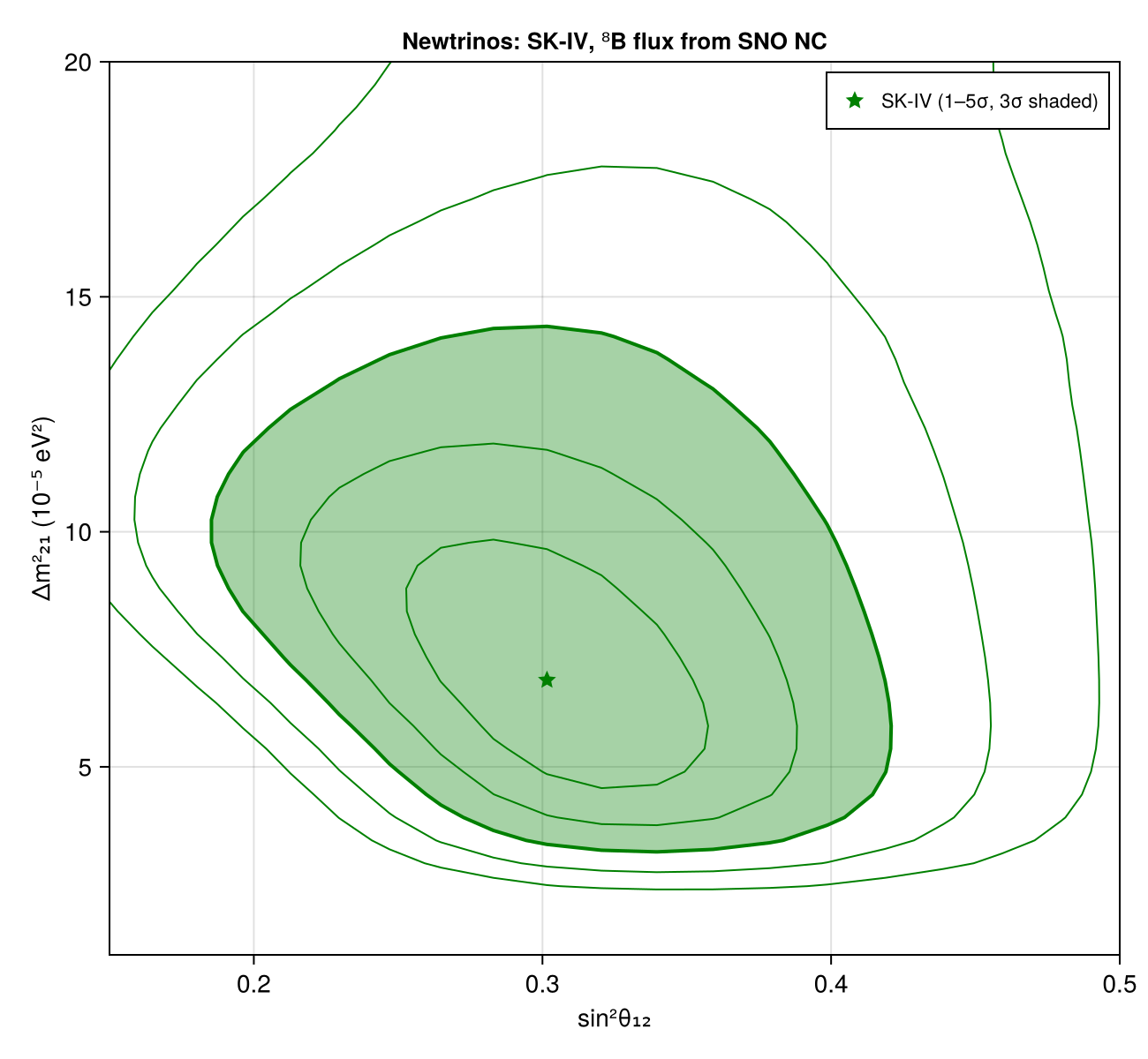
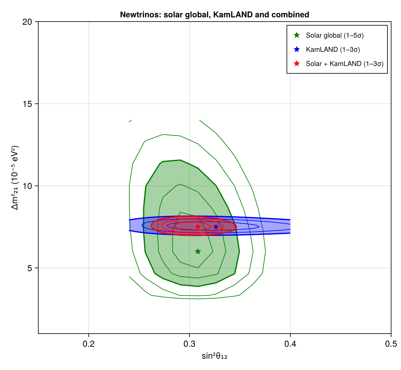
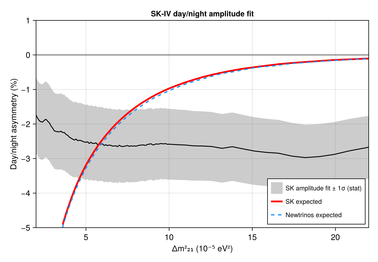
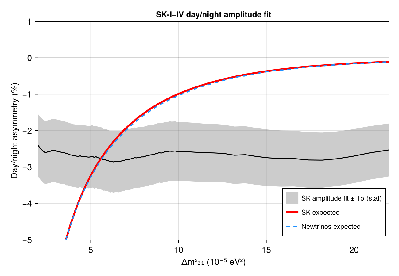
Solar oscillation parameters from Super-Kamiokande IV alone (spectrum plus the day/night amplitude fit, ⁸B flux constrained by SNO's NC measurement), and from the global solar analysis (SK I–IV, SNO, Borexino, radiochemical experiments) compared with and combined with KamLAND, with sin²θ₁₃ = 0.0218; plus the day/night asymmetry from SK's amplitude fit as a function of Δm²₂₁, with the expected asymmetry computed by Newtrinos. On coarse validation grids, Newtrinos finds sin²θ₁₂ = 0.309 [0.272, 0.341], Δm²₂₁ = 6.87 [5.07, 8.71]×10⁻⁵ eV² for SK-IV (SK: 0.308 +0.030/−0.029, 6.90 +1.62/−1.21) and sin²θ₁₂ = 0.303 [0.289, 0.317], Δm²₂₁ = 6.29 [5.52, 7.34]×10⁻⁵ eV² for the solar global fit (SK: 0.306 ± 0.013, 6.10 +0.95/−0.81); with KamLAND (per-period 2013 data) 0.303 [0.291, 0.316] and 7.53 [7.36, 7.71]×10⁻⁵ eV² (SK: 0.307, 7.50); the expected SK-I–IV day/night asymmetry agrees with SK's within 0–3.5 % for Δm²₂₁ = 4–9×10⁻⁵ eV² (Newtrinos slightly larger in magnitude).
Figures
SK-IV: sin²θ₁₂ – Δm²₂₁, 1–5σ · Fig. 39
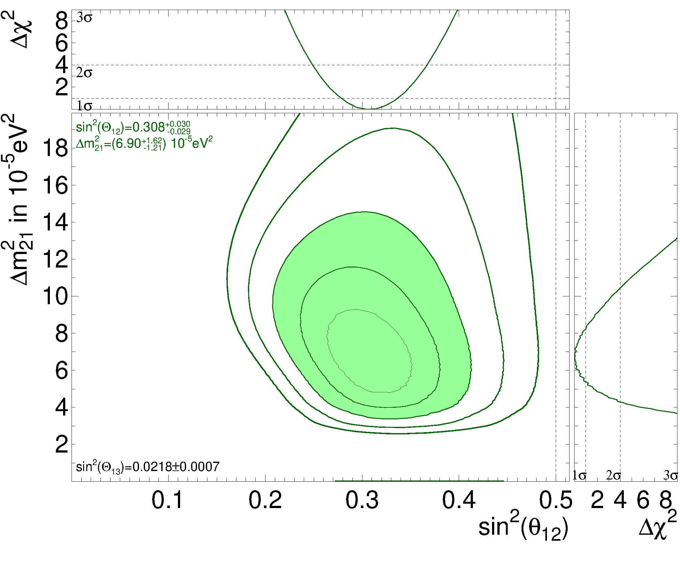
Original figure: Super-Kamiokande, Phys. Rev. D 109, 092001 (2024), Fig. 39, doi:10.1103/PhysRevD.109.092001. Not our work; shown for comparison, all rights with the authors and publisher.
Solar global, KamLAND and combined: sin²θ₁₂ – Δm²₂₁ · Fig. 47
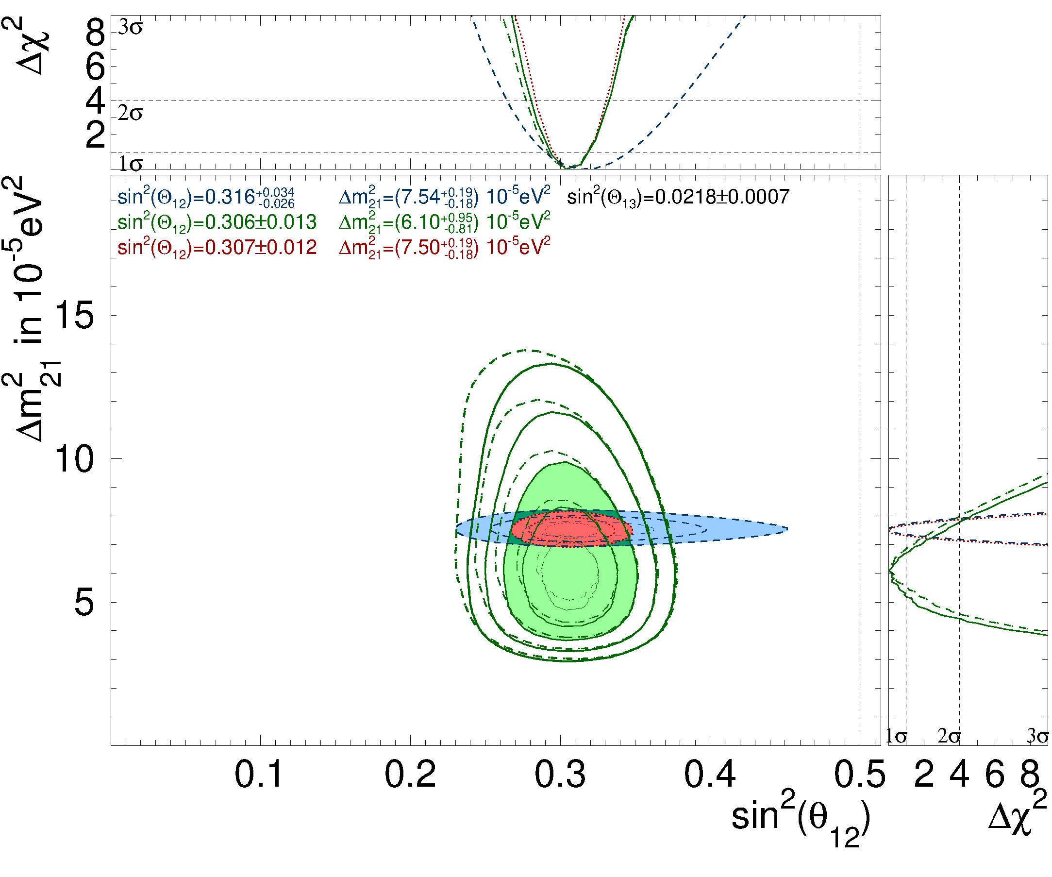
Original figure: Super-Kamiokande, Phys. Rev. D 109, 092001 (2024), Fig. 47, doi:10.1103/PhysRevD.109.092001. Not our work; shown for comparison, all rights with the authors and publisher.
SK-IV day/night amplitude fit vs Δm²₂₁: measured and expected asymmetry · Fig. 49
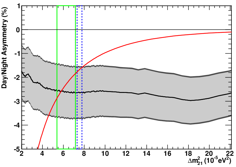
Original figure: Super-Kamiokande, Phys. Rev. D 109, 092001 (2024), Fig. 49, doi:10.1103/PhysRevD.109.092001. Not our work; shown for comparison, all rights with the authors and publisher.
SK-I–IV combined day/night amplitude fit vs Δm²₂₁ · Fig. 52
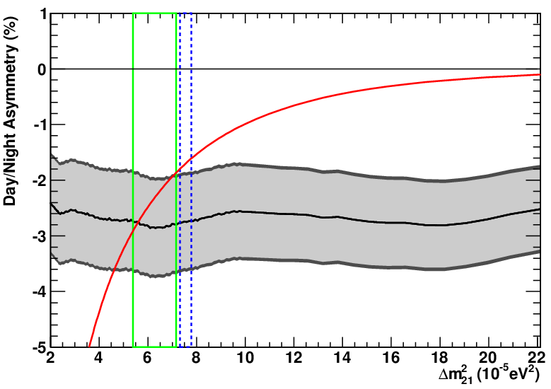
Original figure: Super-Kamiokande, Phys. Rev. D 109, 092001 (2024), Fig. 52, doi:10.1103/PhysRevD.109.092001. Not our work; shown for comparison, all rights with the authors and publisher.
Known limitations
- sin²θ₁₃ is fixed at 0.0218 (SK: Gaussian, ± 0.0007), so that the solar and KamLAND profiles add exactly; the solar + KamLAND region is their sum, with the solar profile spline-interpolated onto KamLAND's finer Δm²₂₁ grid. Coarse validation grids (SK-IV 20×40, global 10×10); intervals from spline-interpolated 1D profiles.
- Day/night: as in SK's analysis, the day/night information enters through SK's amplitude fit of the zenith-angle variation (A_DN vs Δm²₂₁, Figs. 49 and 52, extracted from the vector graphics; module sk_solar_dn), and the published day/night (SK-I: zenith-binned) spectra are merged per energy bin. SK's unbinned time-variation likelihood itself is not public.
- The energy-correlated systematics are modelled with energy-scale and resolution shifts of a Gaussian response and the ⁸B shape uncertainty, not SK's tabulated distortion factors.
- The global solar fit uses the B23 MB22-met solar model with uncorrelated flux priors; SK uses the BP2004/B16 model with its flux covariance and the SK+SNO ⁸B and hep fluxes.
- Borexino enters through its Phase I–II interaction rates and a spectral fit of the Phase-III TFC-subtracted spectrum (backgrounds with Gaussian priors standing in for the non-public tagged spectrum and radial distribution); SK uses only the Phase-II pp, pep and ⁷Be rates.
- The KamLAND curve uses the Newtrinos per-period KamLAND module (2013 data, PRIS reactor fluxes; see the KamLAND PRD 88, 033001 entry), the KamLAND result SK combines with; KamLAND alone gives sin²θ₁₂ = 0.320 [0.291, 0.351] and Δm²₂₁ = 7.54 [7.37, 7.73]×10⁻⁵ eV² at sin²θ₁₃ = 0.0218.
Reproduce
git clone https://github.com/Newtrinos-org/Newtrinos.jl.git && cd Newtrinos.jl && git checkout c6612c255a- Download reproduce.jl into an empty directory.
julia -t 8 --project=/path/to/Newtrinos.jl reproduce.jl
# Reproduction of Super-Kamiokande, Phys. Rev. D 109, 092001 (2024) [arXiv:2312.12907]: solar oscillation analysis
# of SK-IV alone (Fig. 39) and the global solar / KamLAND / combined analysis (Fig. 47), with Newtrinos.jl.
# Run from this directory with the Newtrinos.jl environment at the pinned commit:
#   julia -t 64 --project=<path to Newtrinos.jl> reproduce.jl
using Newtrinos, Distributions, DataStructures, FileIO, CairoMakie, CSV, DataFrames, LinearAlgebra, Interpolations

cd(@__DIR__); mkpath("ours"); mkpath("results"); mkpath("cache")
BLAS.set_num_threads(1)

# CSV export of a profile scan: one row per grid point, ASCII column names, sin²θ, Δm² in eV², dchi2 w.r.t. the best fit
function save_csv(path, r; ref = maximum(r.values.log_posterior))
    ascii(k) = replace(string(k), "θ" => "theta", "Δm²" => "dm2_", "δ" => "d", "₁" => "1", "₂" => "2", "₃" => "3", "CP" => "cp")
    cols = OrderedDict{String,Any}()
    for (k, v) in pairs(r.values)
        x = vec(v)
        startswith(string(k), "θ") && (cols["sin2_" * ascii(k)] = sin.(x) .^ 2)
        cols[ascii(k)] = x
    end
    cols["dchi2"] = 2 .* (ref .- vec(r.values.log_posterior))
    haskey(cols, "llh") && (cols["log_likelihood"] = pop!(cols, "llh"))
    first_cols = filter(in(keys(cols)), ["sin2_theta12", "dm2_21", "dchi2", "log_likelihood", "log_posterior"])
    CSV.write(path, DataFrame(cols)[:, vcat(first_cols, setdiff(collect(keys(cols)), first_cols))])
end

# SK conditions: sin²θ₁₃ = 0.0218 ± 0.0007; here fixed at 0.0218 (the solar and KamLAND data barely constrain it, and
# with θ₁₃ fixed solar and KamLAND share no free parameter besides θ₁₂, Δm²₂₁, so their profiles add); θ₂₃, δCP, Δm²₃₁ fixed
function setup(experiments; extra_priors = (;))
    p = Newtrinos.get_params(experiments)
    priors = Newtrinos.get_priors(experiments)
    θ13 = asin(sqrt(0.0218))
    p = merge(p, (θ₁₃ = θ13, Δm²₂₁ = 7e-5, θ₁₂ = asin(sqrt(0.31))))
    priors = merge(priors, (θ₁₃ = θ13, θ₂₃ = p.θ₂₃, δCP = p.δCP, Δm²₃₁ = p.Δm²₃₁,
                            θ₁₂ = Uniform(asin(sqrt(0.15)), asin(sqrt(0.50))), Δm²₂₁ = Uniform(1e-5, 2e-4)), extra_priors)
    Newtrinos.generate_likelihood(experiments), priors, p
end
# coarse grids: this entry validates the setup, it does not aim at smooth publication-quality contours
grid = OrderedDict(:θ₁₂ => 10, :Δm²₂₁ => 10)

# independent flux normalisations (solar_norm_*), since the SK-IV-only fit constrains ⁸B and hep individually
physics = merge(Newtrinos.solar_common.default_physics(), (solar_flux = Newtrinos.solar_flux.configure(
    Newtrinos.solar_flux.SolarFluxConfig(systematics = Newtrinos.solar_flux.SSMPriors())),))
# as in SK's analysis, the day/night information enters through the amplitude fit of the zenith-angle variation
# (sk_solar_dn), with day and night spectra merged per energy bin
sk_spectra(name) = getproperty(Newtrinos, name).configure(physics; daynight = :combined)
sk4 = (sk4_solar = sk_spectra(:sk4_solar), sk_solar_dn = Newtrinos.sk_solar_dn.configure(physics; dataset = :sk4))
solar = merge(NamedTuple(name => (name in (:sk1_solar, :sk2_solar, :sk3_solar, :sk4_solar) ? sk_spectra(name) :
                                  getproperty(Newtrinos, name).configure(physics))
                         for name in (:chlorine, :gallex_gno, :sage, :sno, :sk1_solar, :sk2_solar, :sk3_solar, :sk4_solar,
                                      :borexino_ph1, :borexino_ph2, :borexino_ph3)),
              (sk_solar_dn = Newtrinos.sk_solar_dn.configure(physics; dataset = :sk1to4),))
kamland = (kamland = Newtrinos.kamland.configure(),)

# Fig. 39: SK-IV alone, ⁸B flux constrained to the SNO NC measurement (5.25 ± 0.20)×10⁶, hep to (7.88 ± 15.76)×10³ /cm²/s
Φ = physics.solar_flux.nominal
flux_sno = (solar_norm_b8 = Truncated(Normal(5.25e6 / Φ.b8, 0.20e6 / Φ.b8), 0.5, 1.5),
            solar_norm_hep = Truncated(Normal(7.88e3 / Φ.hep, 15.76e3 / Φ.hep), 0.0, 10.0))
llh, priors, p = setup(sk4; extra_priors = flux_sno)
# SK-IV alone is cheap: finer grid (the 1D profiles are spline-interpolated for the summary)
r_sk4 = Newtrinos.profile(llh, priors, OrderedDict(:θ₁₂ => 20, :Δm²₂₁ => 40), p, cache_dir = "cache/sk4")
# Fig. 47: all solar data, KamLAND, and both
# the global regions are much smaller: scan a narrower range (same θ₁₂ axis for solar and KamLAND, needed for the sum)
global_range = (θ₁₂ = Uniform(asin(sqrt(0.24)), asin(sqrt(0.40))), Δm²₂₁ = Uniform(2e-5, 14e-5))
llh, priors, p = setup(solar; extra_priors = global_range)
r_solar = Newtrinos.profile(llh, priors, grid, p, cache_dir = "cache/solar")
llh, priors, p = setup(kamland; extra_priors = (θ₁₂ = global_range.θ₁₂,))
# KamLAND fits are cheap; its narrow Δm²₂₁ valley needs the fine grid (same θ₁₂ axis as the solar scan)
r_kl = Newtrinos.profile(llh, priors, OrderedDict(:θ₁₂ => grid[:θ₁₂], :Δm²₂₁ => 191), merge(p, (Δm²₂₁ = 7.5e-5,)), cache_dir = "cache/kamland")

# solar + KamLAND: no shared nuisance parameters, so the combined profile is the sum of the two; the solar profile is
# interpolated (cubic spline in Δm²₂₁) onto the KamLAND grid
function combine(rs, rk; dm_range = (6.5e-5, 8.5e-5))
    @assert rs.axes.θ₁₂ ≈ rk.axes.θ₁₂
    dms_s = range(first(rs.axes.Δm²₂₁), last(rs.axes.Δm²₂₁), length = length(rs.axes.Δm²₂₁))
    @assert collect(dms_s) ≈ rs.axes.Δm²₂₁
    sel = findall(d -> dm_range[1] <= d <= dm_range[2], rk.axes.Δm²₂₁)
    θs, dms = rk.axes.θ₁₂, rk.axes.Δm²₂₁[sel]
    lp = [cubic_spline_interpolation(dms_s, rs.values.log_posterior[i, :])(dms[k]) + rk.values.log_posterior[i, sel[k]]
          for i in eachindex(θs), k in eachindex(dms)]
    (axes = (θ₁₂ = θs, Δm²₂₁ = dms),
     values = (θ₁₂ = [t for t in θs, d in dms], Δm²₂₁ = [d for t in θs, d in dms], log_posterior = lp))
end
r_comb = combine(r_solar, r_kl)

FileIO.save("results/sk4_solar_osc.jld2", Dict("sk4" => r_sk4, "solar" => r_solar, "kamland" => r_kl, "solar_kamland" => r_comb))
save_csv("results/sk4_th12_dm21.csv", r_sk4)
save_csv("results/solar_th12_dm21.csv", r_solar)
save_csv("results/kamland_th12_dm21.csv", r_kl)
save_csv("results/solar_kamland_th12_dm21.csv", r_comb)

Δχ²(r) = 2 .* (maximum(r.values.log_posterior) .- r.values.log_posterior)
s2(r) = sin.(r.axes.θ₁₂) .^ 2
dm(r) = r.axes.Δm²₂₁ .* 1e5
nσ_levels(n) = [quantile(Chisq(2), 1 - 2 * ccdf(Normal(), k)) for k in 1:n]
function bestfit(r)
    i = argmax(r.values.log_posterior)
    s2(r)[i[1]], dm(r)[i[2]]
end
# 1σ interval of a 1D profile (minimum over the other axis)
# from the 1D profile (minimum over the other axis), interpolated with a cubic spline on the uniform scan axis
function interval(x, χ²)
    itp = cubic_spline_interpolation(range(first(x), last(x), length = length(x)), χ²)
    xf = range(first(x), last(x), length = 4001)
    c = itp.(xf)
    inside = xf[c .<= minimum(c) + 1]
    xf[argmin(c)], minimum(inside), maximum(inside)
end

function oscfig(results, title)
    fig = Figure(size = (650, 600))
    ax = Axis(fig[1, 1], title = title, xlabel = "sin²θ₁₂", ylabel = "Δm²₂₁ (10⁻⁵ eV²)", titlesize = 13)
    for (r, color, nσ, fill, label) in results
        lv = nσ_levels(nσ)
        fill && contourf!(ax, s2(r), dm(r), Δχ²(r), levels = [0, lv[3]], colormap = [(color, 0.35)])
        for (k, l) in enumerate(lv)
            contour!(ax, s2(r), dm(r), Δχ²(r), levels = [l], color = color, linewidth = k == 3 ? 2 : 1)
        end
        b = bestfit(r)
        scatter!(ax, [b[1]], [b[2]], color = color, marker = :star5, markersize = 12, label = label)
    end
    xlims!(ax, 0.15, 0.5); ylims!(ax, 1, 20)
    axislegend(ax, position = :rt, labelsize = 11)
    fig
end
save("ours/fig_sk4_th12_dm21.png", oscfig([(r_sk4, :green, 5, true, "SK-IV (1–5σ, 3σ shaded)")], "Newtrinos: SK-IV, ⁸B flux from SNO NC"))
save("ours/fig_global_th12_dm21.png", oscfig([(r_solar, :green, 5, true, "Solar global (1–5σ)"), (r_kl, :blue, 3, true, "KamLAND (1–3σ)"),
                                               (r_comb, :red, 3, true, "Solar + KamLAND (1–3σ)")],
                                              "Newtrinos: solar global, KamLAND and combined"))

# Figs. 49 / 52: day/night amplitude fit vs Δm²₂₁ (SK-IV and SK-I–IV) with the expected asymmetry computed by Newtrinos
function adnfig(dn, title)
    a = dn.assets
    p = merge(Newtrinos.get_params((; dn)), (θ₁₃ = asin(sqrt(0.0218)), θ₁₂ = asin(sqrt(0.31))))
    dms = range(2e-5, 22e-5, length = 81)
    ours = [Newtrinos.sk_solar_dn.expected_adn(merge(p, (Δm²₂₁ = d,)), dn.physics, a) for d in dms]
    CSV.write("results/" * replace(title, r"[^A-Za-z0-9]+" => "_") * ".csv",
              DataFrame(dm2_21 = dms, adn_expected_newtrinos = ours,
                        adn_expected_sk = [Newtrinos.sk_solar_dn.interp(d, a.dm2, a.adn_sk_expected) for d in dms],
                        adn_fit_sk = a.fit_spline.(dms), adn_fit_sigma_stat = a.sigma_spline.(dms)))
    fig = Figure(size = (650, 450))
    ax = Axis(fig[1, 1], title = title, xlabel = "Δm²₂₁ (10⁻⁵ eV²)", ylabel = "Day/night asymmetry (%)", titlesize = 13)
    x = a.dm2 .* 1e5
    band!(ax, x, a.adn_fit .- a.sigma_stat, a.adn_fit .+ a.sigma_stat, color = (:gray, 0.4), label = "SK amplitude fit ± 1σ (stat)")
    lines!(ax, x, a.adn_fit, color = :black)
    lines!(ax, x, a.adn_sk_expected, color = :red, linewidth = 3, label = "SK expected")
    lines!(ax, dms .* 1e5, ours, color = :dodgerblue, linestyle = :dash, linewidth = 2, label = "Newtrinos expected")
    hlines!(ax, [0], color = :black, linewidth = 0.8)
    xlims!(ax, 2, 22); ylims!(ax, -5, 1)
    axislegend(ax, position = :rb, labelsize = 11)
    fig
end
save("ours/fig_sk4_adn_vs_dm2.png", adnfig(sk4.sk_solar_dn, "SK-IV day/night amplitude fit"))
save("ours/fig_sk1to4_adn_vs_dm2.png", adnfig(solar.sk_solar_dn, "SK-I–IV day/night amplitude fit"))

open("results/summary.txt", "w") do io
    for (name, r) in (("SK-IV", r_sk4), ("solar", r_solar), ("KamLAND", r_kl), ("solar+KamLAND", r_comb))
        χ² = Δχ²(r)
        # 1D profiles on the (uniform) scan axes θ₁₂ and Δm²₂₁, then converted
        it = interval(collect(r.axes.θ₁₂), vec(minimum(χ², dims = 2))); id = interval(dm(r), vec(minimum(χ², dims = 1)))
        s2i = sin.(it) .^ 2
        println(io, rpad(name, 15), "sin2_theta12 = ", round(s2i[1], digits = 3), " [", round(s2i[2], digits = 3), ", ", round(s2i[3], digits = 3), "]",
                "   dm2_21 = ", round(id[1], digits = 2), " [", round(id[2], digits = 2), ", ", round(id[3], digits = 2), "] e-5 eV^2")
    end
end
print(read("results/summary.txt", String))
Provenance
| Newtrinos.jl commit | c6612c255a (solar_flux, solar_xsec, solar_common, sk_solar_common, sk_solar_dn, sk1_solar, sk2_solar, sk3_solar, sk4_solar, sno, borexino_ph1, borexino_ph2, borexino_ph3, chlorine, gallex_gno, sage, kamland) |
|---|---|
| Run date | 2026-10-21T17:17:57Z |
| Wall time | 78.0 min (128 threads) |
| Julia | 1.12.5 |
| Machine | AMD EPYC 7702P 64-Core Processor, 128 hardware threads, Linux |
| Environment | newtrinos_Manifest.toml · run.toml |
Downloads
CSV files hold one row per scan point: the scanned and profiled parameters
(sin2_theta23, dm2_32 in eV², dcp in rad, nuisance parameters), dchi2 = −2Δ log L
and the log-likelihood. JLD2 files contain the full NewtrinosResult objects.
| File | Size | SHA-256 |
|---|---|---|
| ours/fig_global_th12_dm21.png | 147.7 kB | 0b62a72fc780… |
| ours/fig_sk1to4_adn_vs_dm2.png | 95.0 kB | 58d31d1621d1… |
| ours/fig_sk4_adn_vs_dm2.png | 100.7 kB | b343e00abba1… |
| ours/fig_sk4_th12_dm21.png | 183.8 kB | a7b427d9705e… |
| results/SK_IV_day_night_amplitude_fit.csv | 6.4 kB | 97edbfde6c39… |
| results/SK_I_IV_day_night_amplitude_fit.csv | 6.4 kB | 545f512ea605… |
| results/kamland_th12_dm21.csv | 598.5 kB | 1c12ae3d99ac… |
| results/sk4_solar_osc.jld2 | 487.8 kB | 93a44b500ca3… |
| results/sk4_th12_dm21.csv | 267.8 kB | d315abfc42b4… |
| results/solar_kamland_th12_dm21.csv | 17.7 kB | 086b6de18d52… |
| results/solar_th12_dm21.csv | 81.4 kB | 1288a3afe2ed… |
| results/summary.txt | 355 B | 9b5bc423a0b2… |