
J. N. Bahcall, P. I. Krastev, A. Yu. Smirnov · Phys. Rev. D 62, 093004 (2000)
SNO: Predictions for ten measurable quantities
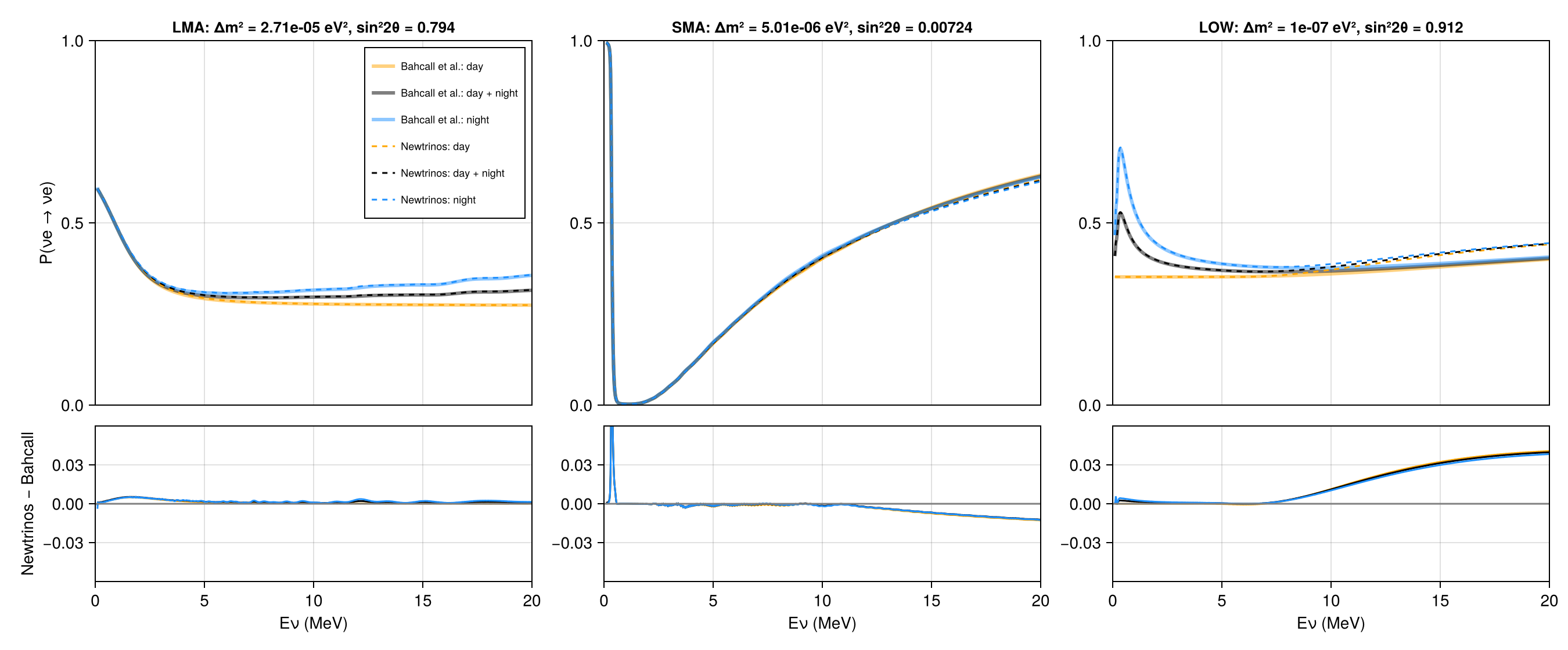
The solar νe survival probability for the two-flavour MSW solutions of 2000, LMA (Δm² = 2.71×10⁻⁵ eV², sin²2θ = 0.794), SMA (5.0×10⁻⁶ eV², 7.2×10⁻³) and LOW (1.0×10⁻⁷ eV², 0.912), averaged over the ⁸B production region and over one year at Sudbury, for day, night and day + night (Fig. 1, numbers from Bahcall's tabulation). It tests the Newtrinos MSW conversion in the Sun, adiabatic (LMA) and non-adiabatic (SMA, LOW: level crossing computed numerically through the solar density profile), and Earth regeneration along PREM chords with the yearly exposure. LMA agrees within 0.005 (day and night) and SMA within 0.013 above 1 MeV; for LOW, Newtrinos is up to 0.04 higher above 10 MeV because Bahcall et al. used the exponential approximation of the solar electron density (with that profile Newtrinos reproduces their LOW values).
Figures
LMA, SMA and LOW survival probabilities vs. neutrino energy (day, night, yearly average) · Fig. 1 (top row)
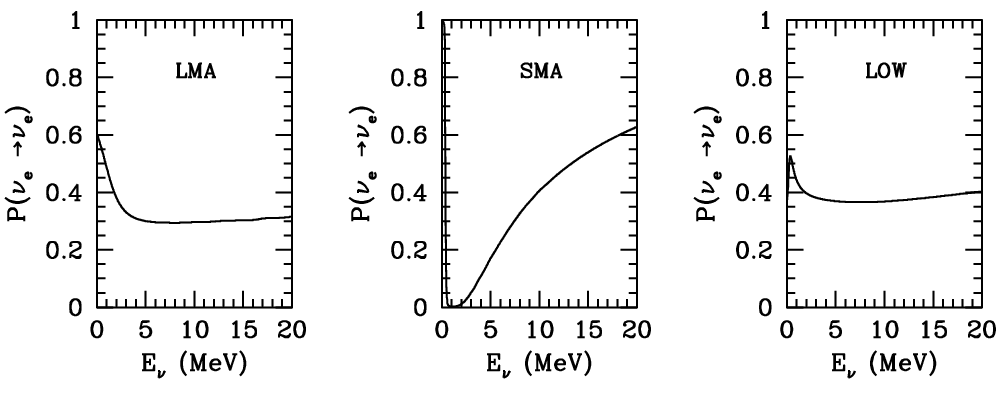
Original figure: J. N. Bahcall, P. I. Krastev, A. Yu. Smirnov, Phys. Rev. D 62, 093004 (2000), Fig. 1 (top row), doi:10.1103/PhysRevD.62.093004. Not our work; shown for comparison, all rights with the authors and publisher.
Known limitations
- Bahcall et al. average over the ⁸B production region of the BP98 solar model; Newtrinos uses B23 (MB22-met). The largest day differences (≤0.005) are in the MSW transition region around 1–3 MeV.
- Earth regeneration: Newtrinos uses PREM with densities averaged along each chord within each of four zones; Bahcall et al. use a detailed Earth model.
- The night average uses 160 bins in cos(zenith). With 40 bins the night probability shows binning wiggles of up to 0.011 at individual energies (3–8 MeV); the Newtrinos solar experiment modules use 20 bins by default, where these wiggles are averaged over the energy spectrum.
- LOW: Bahcall et al. used the exponential approximation n_e = 245 exp(−10.54 r/R☉) N_A/cm³ of the solar electron density, which is less steep than the standard-solar-model profile in the outer Sun where the LOW resonance lies (0.85–0.93 R☉). Newtrinos uses the B23 profile, continued beyond 0.5 R☉ by BS05(OP); run with the exponential profile, its numerical evolution reproduces Bahcall's LOW values (e.g. 0.3761 vs 0.3763 at 14.3 MeV).
- SMA: below 1 MeV the position of the steep MSW threshold depends on the electron density in the ⁸B production region (BP98 vs B23), shifting it by ~3 % in energy (differences up to 0.09 at 0.3–0.4 MeV).
- The vacuum and sterile solutions of the figure are not reproduced; Newtrinos averages the Sun–Earth propagation (no coherent vacuum oscillations, i.e. not valid for Δm² ≲ 10⁻⁹ eV²).
Reproduce
git clone https://github.com/Newtrinos-org/Newtrinos.jl.git && cd Newtrinos.jl && git checkout c6612c255a- Download reproduce.jl and the
data/folder of this entry into an empty directory. julia -t 8 --project=/path/to/Newtrinos.jl reproduce.jl
# Verification of the Newtrinos.jl solar MSW conversion (adiabatic and non-adiabatic) and Earth regeneration against the
# survival probabilities of Bahcall, Krastev & Smirnov, Phys. Rev. D 62, 093004 (2000), Fig. 1 (LMA, SMA and LOW panels),
# tabulated by Bahcall in data/Psurv_*.dat (day, day + night and night, averaged over one year and over the ⁸B production
# region; the two-flavour parameters are given at the end of each file).
# Run from this directory with the Newtrinos.jl environment at the pinned commit:
#   julia -t 8 --project=<path to Newtrinos.jl> reproduce.jl
using Newtrinos, CairoMakie, CSV, DataFrames, DelimitedFiles, Printf

cd(@__DIR__); mkpath("ours"); mkpath("results")
physics = Newtrinos.solar_common.default_physics()
p0 = Newtrinos.get_params((chlorine = Newtrinos.chlorine.configure(physics),))
# Sudbury (46.3° N, SNO at 2 km depth); regeneration computed at all energies; 160 night bins in cos(zenith): with
# coarse bins (the experiment modules use 20) the night probability shows binning wiggles of up to ~0.01
site = Newtrinos.solar_common.Site(physics, 46.3; depth_km = 2.0, n_night = 160, E_night_min = 0.0)

function read_bahcall(sol)
    lines = readlines("data/Psurv_$sol.dat")
    rows = [parse.(Float64, split(l)) for l in lines if occursin(r"^\s*[0-9]\.[0-9]+E[+-][0-9]+\s", l)]
    par = match(r"sin2theta\s*=\s*(\S+)\s+dm2\s*=\s*(\S+)", join(lines, " "))
    reduce(vcat, permutedims.(rows)), parse(Float64, par[1]), parse(Float64, par[2])
end

fig = Figure(size = (1350, 560))
for (k, sol) in enumerate(("LMA", "SMA", "LOW"))
    ref, s22, dm2 = read_bahcall(sol)
    E = ref[:, 1]
    p = merge(p0, (θ₁₂ = asin(sqrt(s22)) / 2, θ₁₃ = 0.0, Δm²₂₁ = dm2))
    P = Newtrinos.solar_common.survival(physics, site, :b8, E, p)
    day = P.day[:, 1]
    night = vec(sum(P.night[:, :, 1] .* site.w_night', dims = 2)) ./ sum(site.w_night)
    avg = site.w_day .* day .+ sum(site.w_night) .* night
    CSV.write("results/survival_$(lowercase(sol)).csv",
              DataFrame(E_MeV = E, day_newtrinos = day, day_bahcall = ref[:, 2], avg_newtrinos = avg, avg_bahcall = ref[:, 3],
                        night_newtrinos = night, night_bahcall = ref[:, 4]))
    above = E .>= 1.0
    @printf("%s (sin²2θ = %.4g, Δm² = %.4g eV²): max |Δ| day %.4f, night %.4f (all E); above 1 MeV day %.4f, night %.4f\n",
            sol, s22, dm2, maximum(abs.(day .- ref[:, 2])), maximum(abs.(night .- ref[:, 4])),
            maximum(abs.(day[above] .- ref[above, 2])), maximum(abs.(night[above] .- ref[above, 4])))
    ax = Axis(fig[1, k], ylabel = k == 1 ? "P(νe → νe)" : "", titlesize = 13,
              title = @sprintf("%s: Δm² = %.3g eV², sin²2θ = %.3g", sol, dm2, s22))
    for (lab, col, c) in (("day", 2, :orange), ("day + night", 3, :black), ("night", 4, :dodgerblue))
        lines!(ax, E, ref[:, col], color = c, linewidth = 3, alpha = 0.5, label = "Bahcall et al.: $lab")
    end
    lines!(ax, E, day, color = :orange, linestyle = :dash, label = "Newtrinos: day")
    lines!(ax, E, avg, color = :black, linestyle = :dash, label = "Newtrinos: day + night")
    lines!(ax, E, night, color = :dodgerblue, linestyle = :dash, label = "Newtrinos: night")
    xlims!(ax, 0, 20); ylims!(ax, 0, 1); hidexdecorations!(ax, grid = false)
    k == 1 && axislegend(ax, position = :rt, labelsize = 9)
    axr = Axis(fig[2, k], xlabel = "Eν (MeV)", ylabel = k == 1 ? "Newtrinos − Bahcall" : "")
    lines!(axr, E, day .- ref[:, 2], color = :orange); lines!(axr, E, avg .- ref[:, 3], color = :black)
    lines!(axr, E, night .- ref[:, 4], color = :dodgerblue)
    hlines!(axr, [0], color = :gray); xlims!(axr, 0, 20); ylims!(axr, -0.06, 0.06)
end
rowsize!(fig.layout, 2, Relative(0.3))
save("ours/fig_survival_msw.png", fig)
Provenance
| Newtrinos.jl commit | c6612c255a (osc, solar_flux, earth_layers, solar_common) |
|---|---|
| Run date | 2026-10-21T16:43:45Z |
| Wall time | 3.9 min (128 threads) |
| Julia | 1.12.5 |
| Machine | AMD EPYC 7702P 64-Core Processor, 128 hardware threads, Linux |
| Environment | newtrinos_Manifest.toml · run.toml |
Downloads
CSV files hold one row per scan point: the scanned and profiled parameters
(sin2_theta23, dm2_32 in eV², dcp in rad, nuisance parameters), dchi2 = −2Δ log L
and the log-likelihood. JLD2 files contain the full NewtrinosResult objects.
| File | Size | SHA-256 |
|---|---|---|
| ours/fig_survival_msw.png | 239.4 kB | 7c86698cc880… |
| results/survival_lma.csv | 81.9 kB | 669361756935… |
| results/survival_low.csv | 81.9 kB | 244529dbf343… |
| results/survival_sma.csv | 82.8 kB | f8720a44ab14… |