
G. L. Fogli, E. Lisi, D. Montanino, A. Palazzo · Phys. Rev. D 62, 113004 (2000)
Quasi-vacuum solar neutrino oscillations
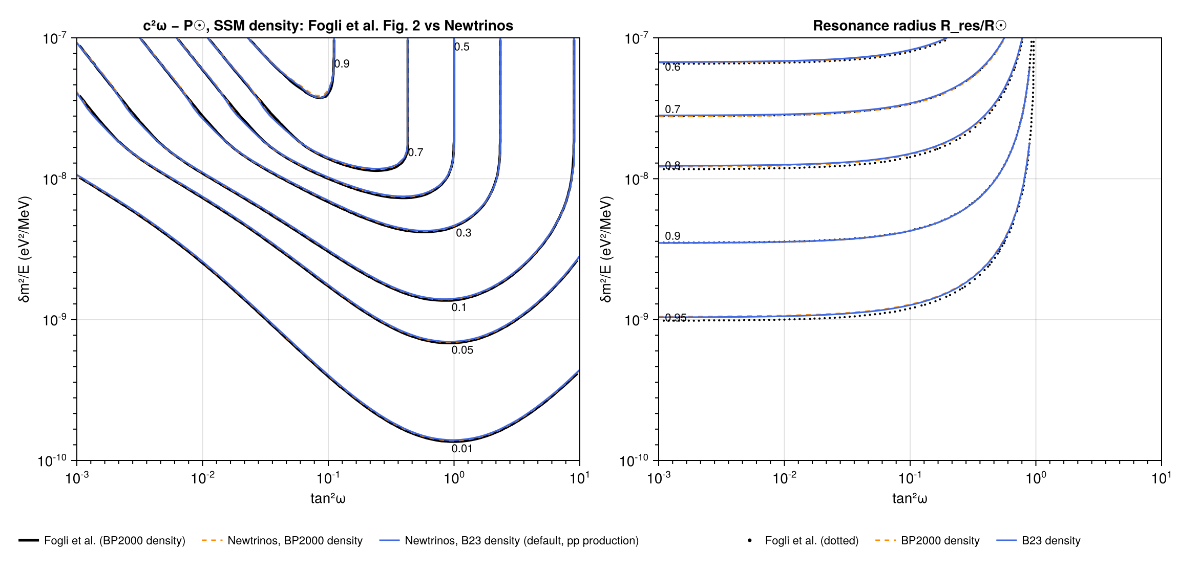
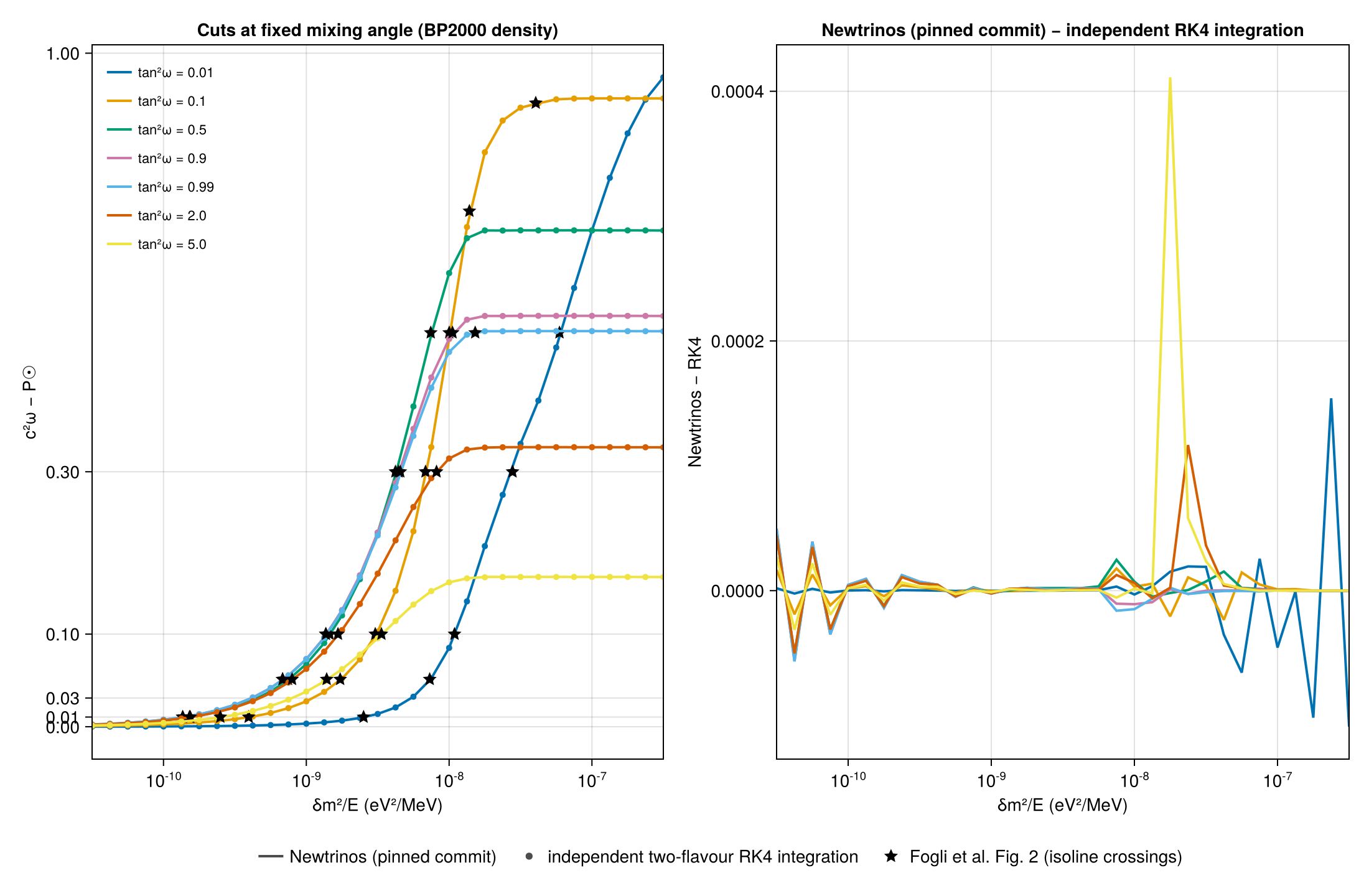
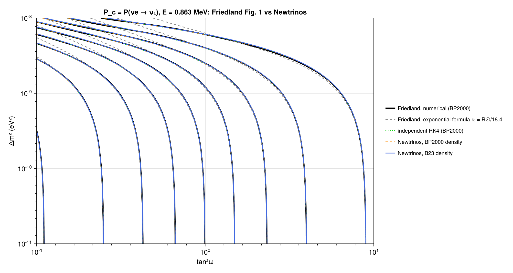
The conversion of solar νe in the Sun for 10⁻¹⁰ ≲ δm²/E ≲ 10⁻⁷ eV²/MeV, where it is neither vacuum-like nor adiabatic: the correction c²ω − P☉ (P☉ = P(νe → ν₁) at the solar surface) in the full mixing plane for the standard solar model and for the exponential density (Figs. 2, 3), the Earth correction (Fig. 4), the level-crossing probability at the ⁷Be energy in both octants (Friedland, Fig. 1), and the interference term that the averaged Sun–Earth propagation drops. Newtrinos is also compared with an independent two-flavour integration of the evolution equation (RK4), with both the B23 and the BP2000 density (the one used in the papers). Newtrinos reproduces Fig. 2 along its isolines within ~2 % and agrees with the RK4 integration within 4×10⁻⁴ in both octants and at maximal mixing (B23 vs BP2000: ≤ 0.006); Friedland's P_c isolines are reproduced within 0.01 for θ < 45° and 0.003 for θ > 45°; its Parke formula reproduces the semianalytical Fig. 3 exactly, and the Earth correction agrees within ~3 % (medians along the isolines). The comparison led to a fix of the level crossing for θ > 45° and near maximal mixing (Newtrinos f64fa41). Not covered: the coherent Sun–Earth interference term, which Newtrinos averages out (valid for Δm² ≳ 10⁻⁸ eV² for the ⁷Be and pep lines).
Figures
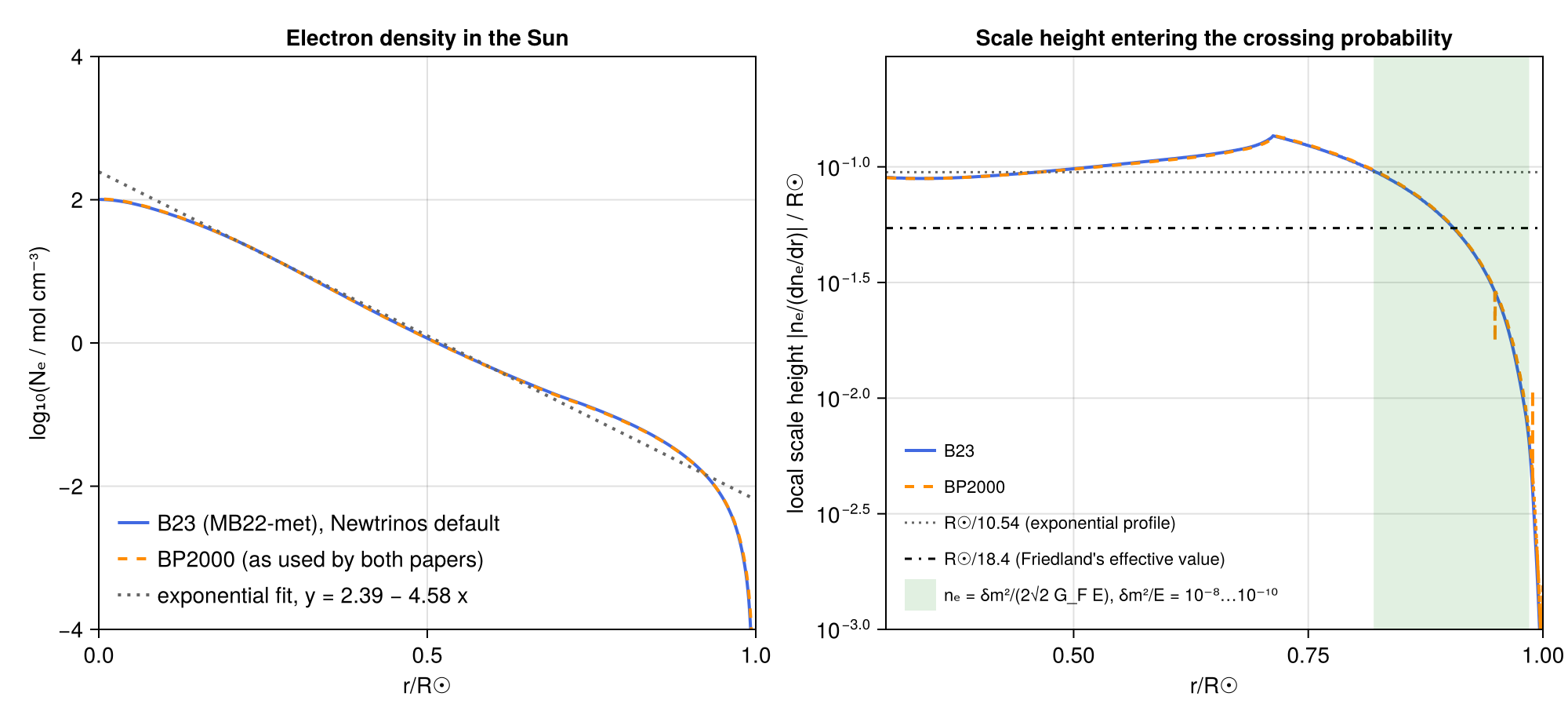
Solar electron density (B23, BP2000, exponential fit) and its local scale height, with the region where the quasi-vacuum conversion happens · Fig. 1
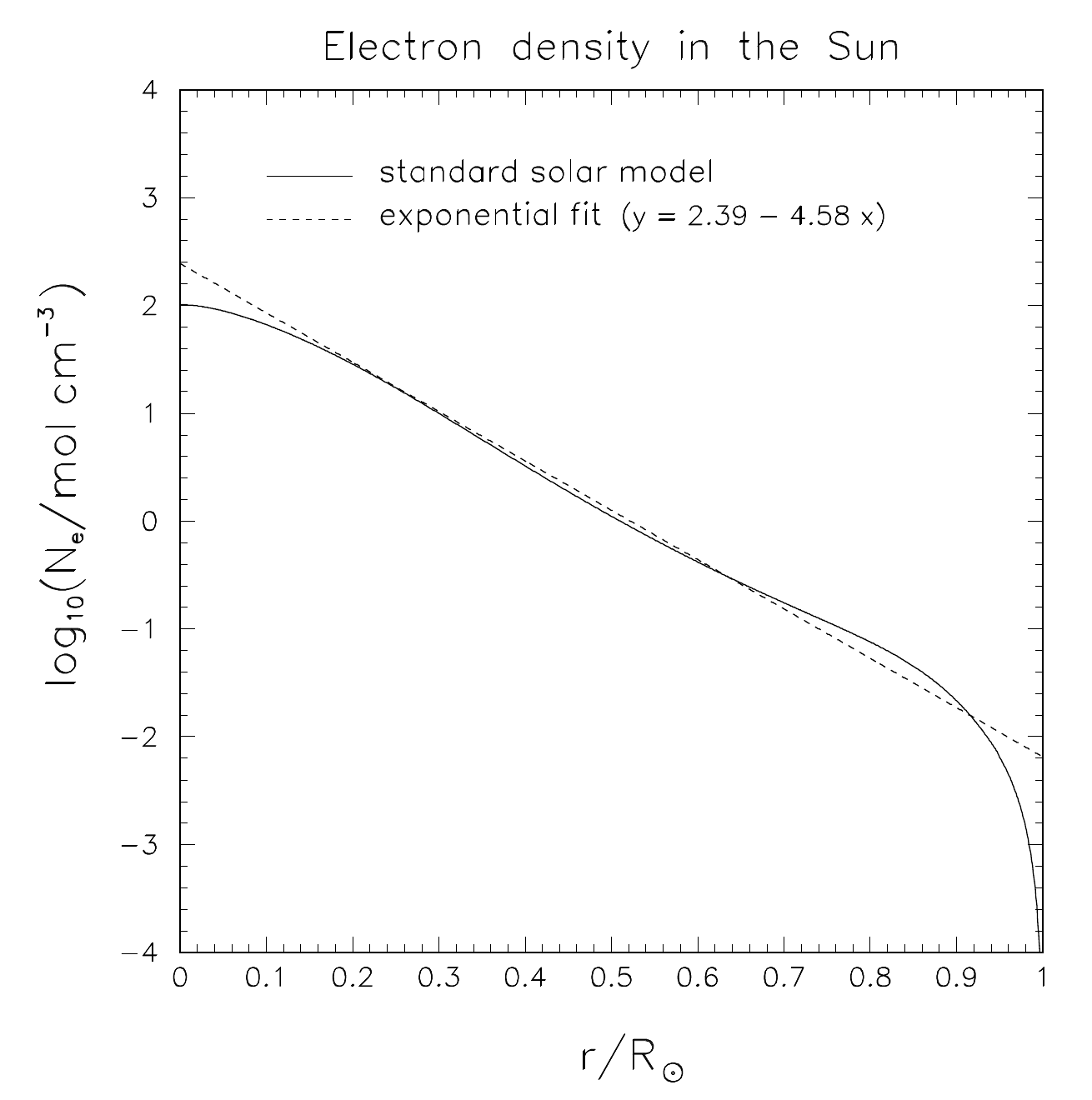
Original figure: G. L. Fogli, E. Lisi, D. Montanino, A. Palazzo, Phys. Rev. D 62, 113004 (2000), Fig. 1, doi:10.1103/PhysRevD.62.113004. Not our work; shown for comparison, all rights with the authors and publisher.
Isolines of c²ω − P☉ for the solar-model density, and resonance radii: Fogli et al. vs Newtrinos (BP2000 and B23 density) · Fig. 2
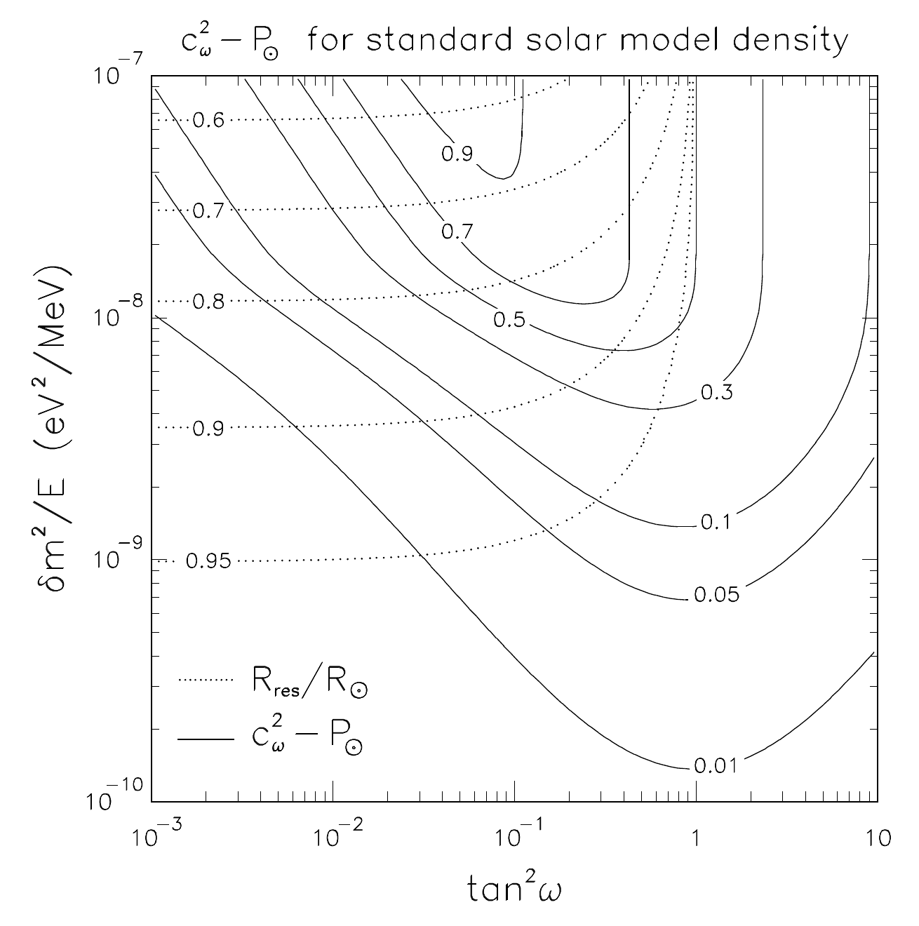
Original figure: G. L. Fogli, E. Lisi, D. Montanino, A. Palazzo, Phys. Rev. D 62, 113004 (2000), Fig. 2, doi:10.1103/PhysRevD.62.113004. Not our work; shown for comparison, all rights with the authors and publisher.
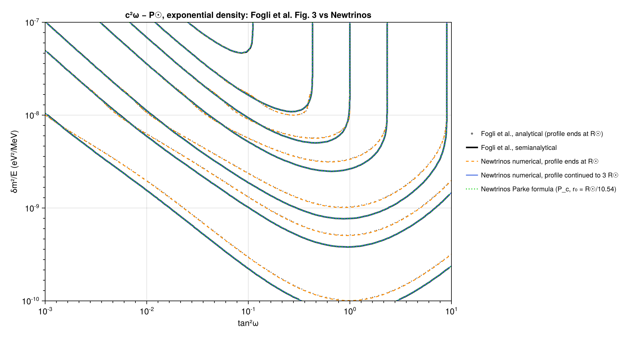
Isolines of c²ω − P☉ for the exponential density: analytical and semianalytical (Fogli et al.) vs Newtrinos numerical evolution and Parke formula · Fig. 3
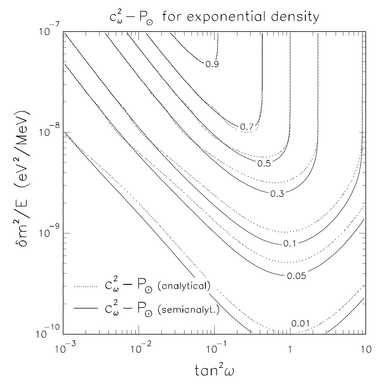
Original figure: G. L. Fogli, E. Lisi, D. Montanino, A. Palazzo, Phys. Rev. D 62, 113004 (2000), Fig. 3, doi:10.1103/PhysRevD.62.113004. Not our work; shown for comparison, all rights with the authors and publisher.
c²ω − P☉ at fixed mixing angle in both octants: Newtrinos vs an independent RK4 integration vs the Fig. 2 isolines · Fig. 2 (sections)
Fig. 2 (sections)
Level-crossing probability at the ⁷Be energy in both octants: Friedland (BP2000 numerical, exponential r₀ = R☉/18.4) vs RK4 and Newtrinos · Friedland, PRL 85, 936, Fig. 1
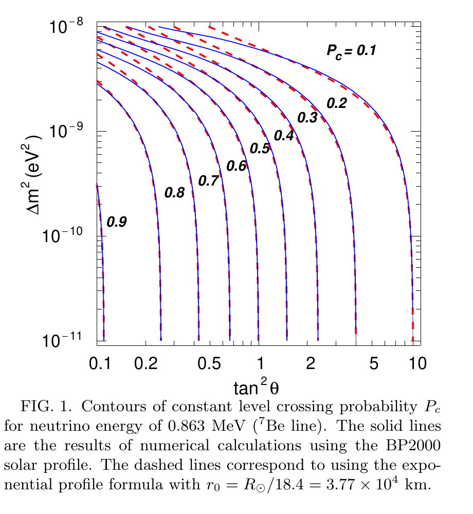
Original figure: G. L. Fogli, E. Lisi, D. Montanino, A. Palazzo, Phys. Rev. D 62, 113004 (2000), Friedland, PRL 85, 936, Fig. 1, doi:10.1103/PhysRevD.62.113004. Not our work; shown for comparison, all rights with the authors and publisher.
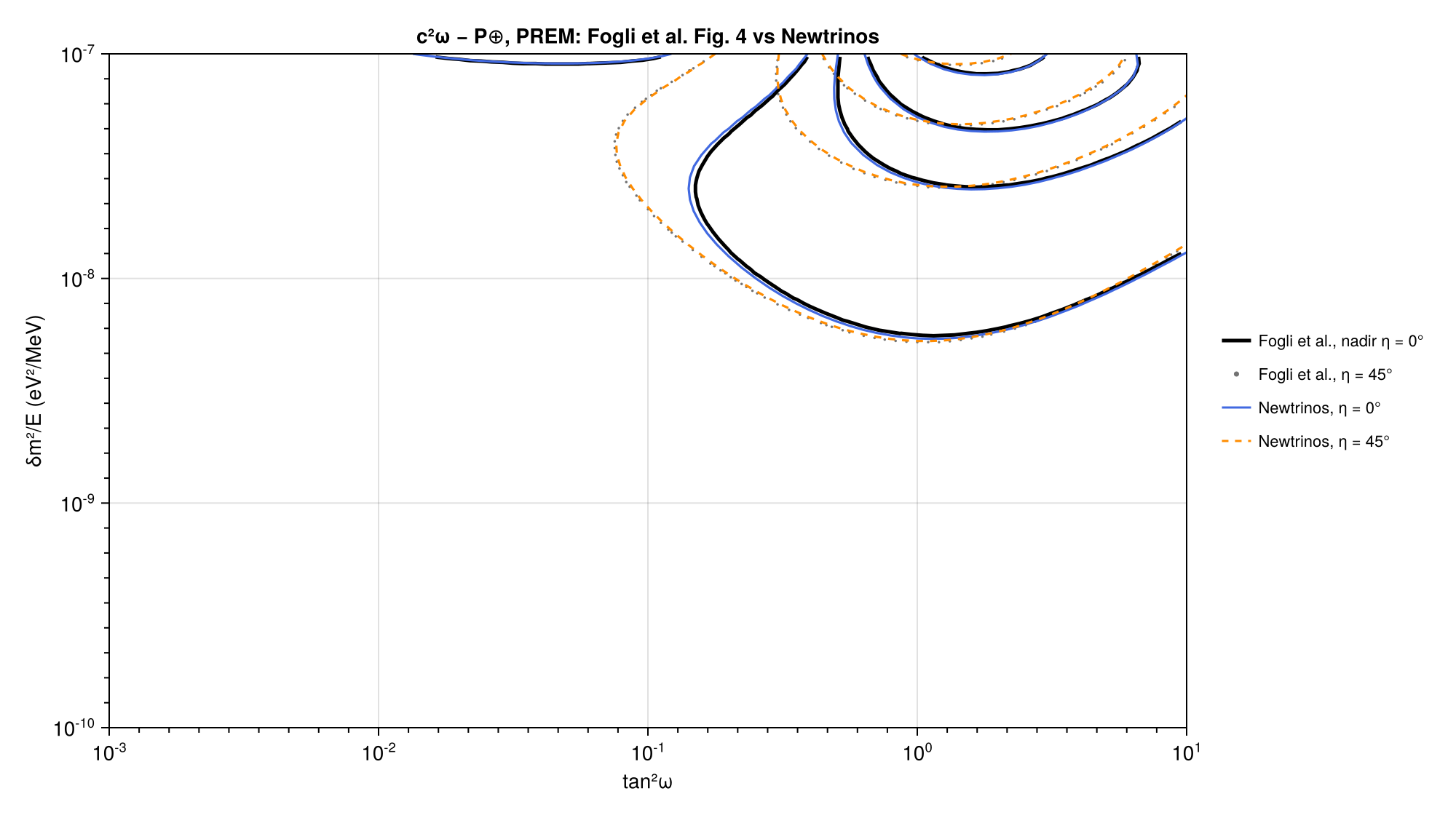
Isolines of the Earth correction c²ω − P⊕ (PREM) for nadir angles 0° and 45° · Fig. 4
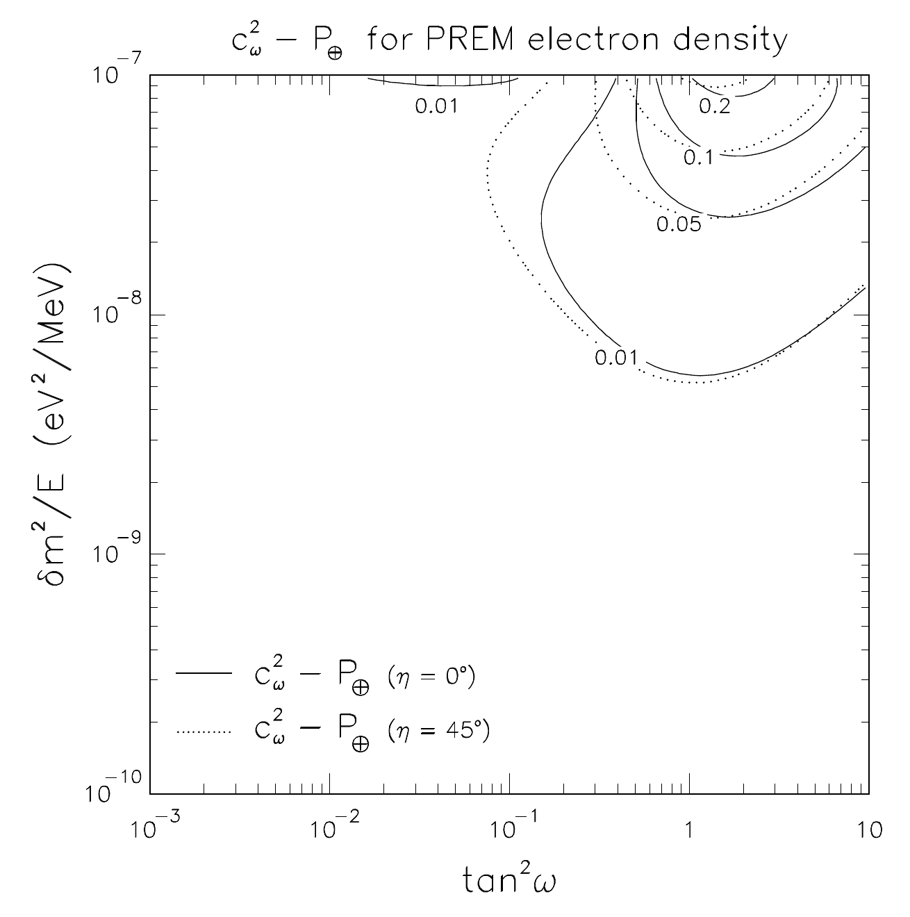
Original figure: G. L. Fogli, E. Lisi, D. Montanino, A. Palazzo, Phys. Rev. D 62, 113004 (2000), Fig. 4, doi:10.1103/PhysRevD.62.113004. Not our work; shown for comparison, all rights with the authors and publisher.
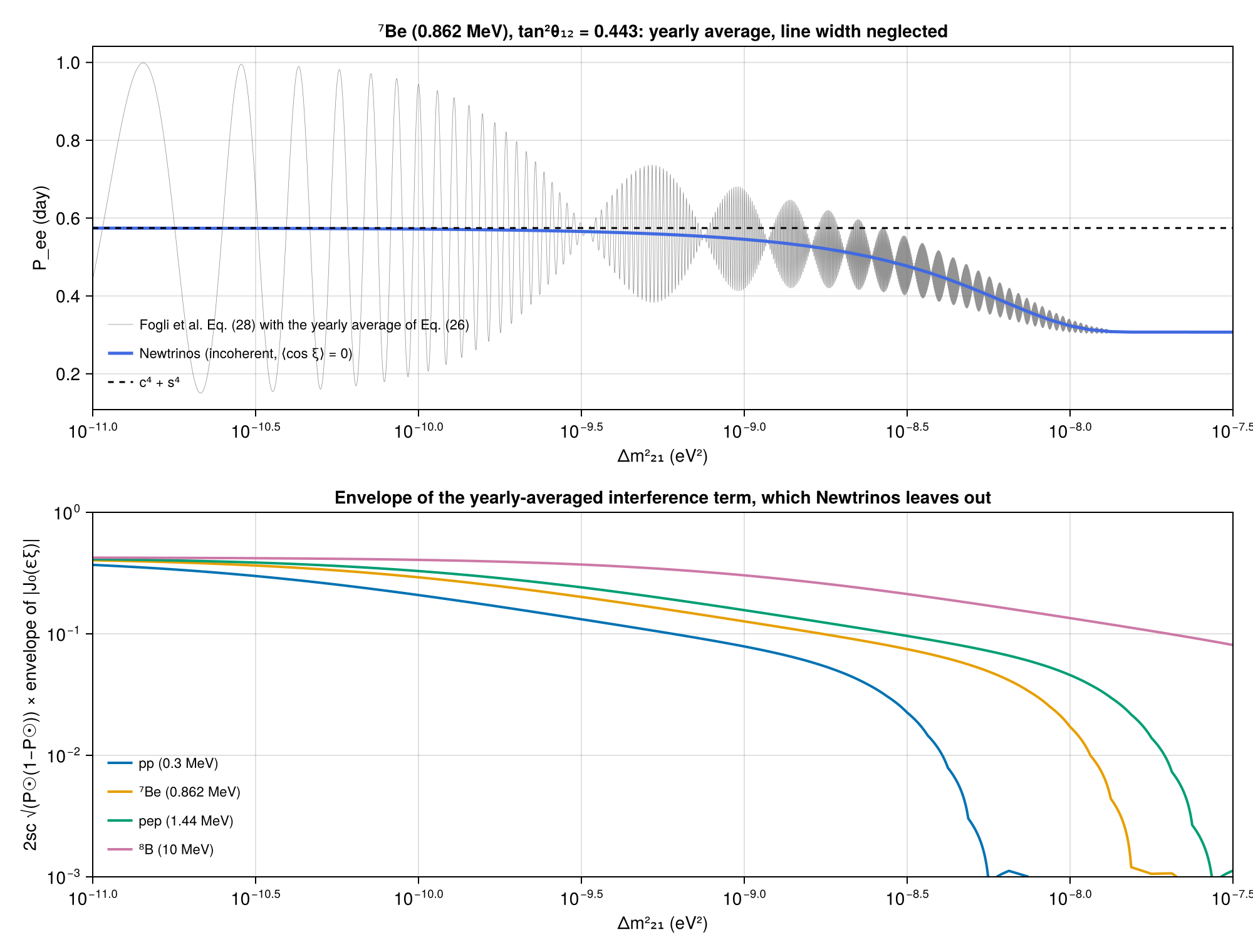
The interference term of Eq. (28) left out by the averaged Sun–Earth propagation: ⁷Be P_ee with the yearly average (Eq. 26), and its amplitude for line energies · Eqs. (26), (28)
Eqs. (26), (28)
Known limitations
- Before Newtrinos f64fa41 (e.g. 09ed1fe), the level crossing was wrong in two cases. (1) θ > 45°:
solar_crossing_probabilityreturned P_c = 0 for cos 2θ ≤ 0 (no resonance) and the conversion was treated as adiabatic, e.g. c²ω − P☉ = 0.333 (0.167) instead of 0.061 (0.037) at tan²ω = 2 (5) and δm²/E = 10⁻⁹ eV²/MeV; Friedland's P_c = 0.1–0.4 isolines came out as 0. (2) Near maximal mixing the numerical evolution started at 1000 × the resonance density, which vanishes as cos 2θ → 0: |Newtrinos − RK4| was 0.007 at tan²ω = 0.9 and 0.095 at 0.99 (≤ 3×10⁻⁴ for tan²ω ≤ 0.5); a profile ending above the resonance density (exponential profile cut at R☉, δm²/E ≲ 10⁻⁹) was likewise treated as adiabatic. Both only affect Δm²₂₁ ≲ 10⁻⁷ eV² (not LMA). Since f64fa41 the scale height for Parke's formula (which holds in both octants) is taken at |cos 2θ| n_* (n_* = Δm²/(2E√2 G_F c₁₃²), floor 10⁻² n_*, outermost interval beyond the table) and the numerical evolution starts at 1000 n_*; solar regression references were unchanged by this change. - Newtrinos averages the Sun–Earth propagation: P_ee = Σᵢ P(νe → νᵢ)|U_ei|², i.e. Fogli et al.'s Eq. (28) without the interference term 2 s c √(P☉(1−P☉)) cos ξ. The yearly average alone (Eq. 26) damps it only like |J₀(εξ)| ~ (εξ)^(−1/2): for a monoenergetic line its amplitude is still 0.13 (⁷Be) and 0.16 (pep) at Δm² = 10⁻⁹ eV², and 0.017 / 0.046 at 10⁻⁸ eV². The thermal line width (Fogli et al. Fig. 5, not reproduced) removes it for δm²/E ≳ 10⁻⁸ eV²/MeV, and energy integration of continuous spectra removes it at lower δm²/E. The Newtrinos solar code comment states validity for Δm² ≳ 10⁻⁹ eV²; for the ⁷Be and pep lines the averaging is accurate only for Δm² ≳ 10⁻⁸ eV². No vacuum/just-so solution can be fitted with Newtrinos.
- Fogli et al. used the BP2000 ('year 2000') electron density (Bahcall's neordered.output, in data/); Newtrinos uses B23. The two agree within ~2 % up to 0.95 R☉ and 10 % at 0.98 R☉, and the correction c²ω − P☉ differs by ≤ 0.006 between them; the comparisons with the paper are therefore made with both. The non-adiabatic region (nₑ ≈ δm²/(2√2 G_F E)) lies at 0.82–0.985 R☉ for δm²/E = 10⁻⁸–10⁻¹⁰ eV²/MeV, where the local scale height falls from R☉/10 to below R☉/100 (Friedland's effective R☉/18.4 is reached at ~0.91 R☉).
- Fogli et al. quote that at tan²ω ≃ 1 the correction reaches 0.05 at δm²/E ≃ 8×10⁻¹⁰ eV²/MeV for the true density and ~2× lower for the exponential one. Their Fig. 2 isoline is at 6.8×10⁻¹⁰; the RK4 integration gives 6.9×10⁻¹⁰ (BP2000), 7.0×10⁻¹⁰ (B23), 5.1×10⁻¹⁰ (exponential ending at R☉), Newtrinos 6.9×10⁻¹⁰ (BP2000, tan²ω = 0.99) and the semianalytical formula 3.8×10⁻¹⁰.
- The paper curves were digitised from the vector graphics of the arXiv versions (data/). The isoline levels of the solid lines are those printed in the figures; the dotted lines (Fig. 2 resonance radii, Fig. 3 analytical, Fig. 4 at η = 45°) are unlabelled dots and are compared by evaluating Newtrinos at each dot. Fig. 3 'analytical' (exponential profile up to R☉, vacuum outside) is compared with the Newtrinos numerical evolution through that profile (within 0.5 % median / 1.5 % at the 90th percentile of the nearest level); Newtrinos has no hypergeometric-function solution. The Fig. 2 isoline statistics use tan²ω < 0.9; the second octant is tested with the cuts (RK4) and Friedland's figure.
- Earth (Fig. 4): Newtrinos uses
PREM_discontinuitieswith chord-averaged densities (as the solar experiment modules), Fogli et al. a five-step biquadratic PREM with a first-order perturbative evolution. The two-flavour limit is taken as θ₁₃ = 0 (ν₃ decouples exactly). The three-flavour analysis (Figs. 6–8) is not reproduced.
Reproduce
git clone https://github.com/Newtrinos-org/Newtrinos.jl.git && cd Newtrinos.jl && git checkout aa98e0c218- Download reproduce.jl and the
data/folder of this entry into an empty directory. julia -t 8 --project=/path/to/Newtrinos.jl reproduce.jl
# Verification of the Newtrinos.jl conversion of solar neutrinos in the Sun (module `osc`: `solar_mass_fractions`,
# `solar_transition_matrix`, `solar_crossing_probability`; solar density profile from `solar_flux`) in the
# quasi-vacuum regime, 10⁻¹⁰ ≲ δm²/E ≲ 10⁻⁷ eV²/MeV, against
#   G.L. Fogli, E. Lisi, D. Montanino, A. Palazzo, "Quasi-vacuum solar neutrino oscillations", PRD 62, 113004 (2000)
#   A. Friedland, "MSW effects in vacuum oscillations", PRL 85, 936 (2000)
# and against an independent two-flavour integration of the evolution equation (RK4, below).
# Run from this directory with the Newtrinos.jl environment at the pinned commit:
#   julia -t 8 --project=<path to Newtrinos.jl> reproduce.jl
using Newtrinos, CairoMakie, DelimitedFiles, LinearAlgebra, Printf, SpecialFunctions, Statistics

cd(@__DIR__); mkpath("ours"); mkpath("results")

const O = Newtrinos.osc
const SF = Newtrinos.solar_flux
const EL = Newtrinos.earth_layers

const sf = SF.configure()
const cfg = O.OscillationConfig(flavour = O.ThreeFlavour(), interaction = O.SI())
# two-flavour limit of the papers: θ₁₃ = 0 decouples ν₃ exactly
const p0 = merge(O.configure(cfg).params, (θ₁₃ = 0.0,))

# ------------------------------------------------------------------------------------------------
# electron density profiles (r in R☉, nₑ in mol/cm³)
# ------------------------------------------------------------------------------------------------
const B23 = sf.production.pp.profile            # Newtrinos default: B23 (MB22-met), centre to surface
function read_bp2000()
    d = readdlm("data/bp2000_ne.csv", ',', Float64; skipstart = 3)
    o = sortperm(d[:, 1]); r = d[o, 1]; ne = 10 .^ d[o, 2]
    keep = [true; diff(r) .> 0]
    (r = r[keep], ne = ne[keep], nn = ne[keep] ./ 2)
end
const BP2000 = read_bp2000()                    # the "year 2000" SSM profile used by both papers
# exponential approximation of Fogli et al. (Bahcall 1989): Nₑ = 245 exp(-10.54 r/R☉) mol/cm³, up to r_max
function exp_profile(r_max)
    r = collect(range(0, r_max, length = round(Int, 1000r_max) + 1))
    (r = r, ne = 245.0 .* exp.(-10.54 .* r), nn = 122.5 .* exp.(-10.54 .* r))
end
const EXP1 = exp_profile(1.0)   # ends at the solar radius (vacuum outside): the "analytical" case of Fogli et al.
const EXP3 = exp_profile(3.0)   # continued far beyond R☉: the limit of their "semianalytical" approximation

function ne_at(prof, x)
    i = clamp(searchsortedlast(prof.r, x), 1, length(prof.r) - 1)
    t = (x - prof.r[i]) / (prof.r[i+1] - prof.r[i])
    exp(log(prof.ne[i]) + t * (log(prof.ne[i+1]) - log(prof.ne[i])))
end
# radius at which nₑ = n (outermost crossing), and local scale height |nₑ/(dnₑ/dr)| in R☉
r_at(prof, n) = (i = findfirst(<(n), prof.ne); i === nothing || i == 1 ? NaN :
                 prof.r[i-1] + log(prof.ne[i-1] / n) / log(prof.ne[i-1] / prof.ne[i]) * (prof.r[i] - prof.r[i-1]))
scale_height(prof) = (r = (prof.r[1:end-1] .+ prof.r[2:end]) ./ 2, h = diff(prof.r) ./ log.(prof.ne[1:end-1] ./ prof.ne[2:end]))

# single production point (Fogli et al.: in the QV regime P_sun does not depend on the production point)
production_at(prof, r = 0.1) = (r = [r], ne = [ne_at(prof, r)], nn = [ne_at(prof, r) / 2], w = [1.0], profile = prof)

# ------------------------------------------------------------------------------------------------
# Newtrinos: P_sun = P(νe → ν₁) at the solar surface, P_earth = P(ν₁ → νe) at the detector
# ------------------------------------------------------------------------------------------------
θ_of(tan2) = atan(sqrt(tan2))
matrices(tan2, dm2) = O._solar_matrices(cfg, merge(p0, (θ₁₂ = θ_of(tan2), Δm²₂₁ = dm2)))
function psun(tan2, dm2, E_MeV, production)
    U, h = matrices(tan2, dm2)
    O.solar_mass_fractions(U, h, [E_MeV * 1e-3], production, O.SI())[1, 1]
end
# Newtrinos' estimate of the crossing probability (Parke's formula with the local scale height of `profile`)
function pc_parke(tan2, dm2, E_MeV, ne_prod, profile)
    U, h = matrices(tan2, dm2)
    O.solar_crossing_probability(h[2] - h[1], abs2(U[1, 1]), abs2(U[1, 2]), E_MeV * 1e-3, ne_prod, profile)
end

# ------------------------------------------------------------------------------------------------
# independent reference: two-flavour evolution equation integrated with RK4 (fixed phase per step),
# from the matter eigenstates at r_prod (populations cos²θm, sin²θm) to the end of the profile
# ------------------------------------------------------------------------------------------------
const HBARC = 1.973269804e-7                    # eV m
const RSUN = 6.957e8                            # m
const VCC = sqrt(2) * 1.1663788e-23 * (HBARC * 100)^3 * 6.02214076e23   # √2 G_F N_A [eV cm³]
function psun_rk4(tan2, dm2, E_MeV, prof; r_prod = 0.1, dphi = 0.02)
    θ = θ_of(tan2); c2θ, s2θ = cos(2θ), sin(2θ)
    δ = dm2 / (2E_MeV * 1e6)
    k = RSUN / HBARC
    H(r) = (V = VCC * ne_at(prof, r); [(-δ*c2θ/2 + V) (δ*s2θ/2); (δ*s2θ/2) (δ*c2θ/2)])
    Um = eigen(Hermitian(H(r_prod))).vectors
    ψ = ComplexF64.(Um)
    f(r, ψ) = -im * k .* (H(r) * ψ)
    r = r_prod; rend = prof.r[end]
    while r < rend
        V = VCC * ne_at(prof, r)
        hs = min(dphi / (k * sqrt((V - δ * c2θ)^2 + (δ * s2θ)^2)), 1e-3, rend - r)
        k1 = f(r, ψ); k2 = f(r + hs / 2, ψ + hs / 2 * k1); k3 = f(r + hs / 2, ψ + hs / 2 * k2); k4 = f(r + hs, ψ + hs * k3)
        ψ += hs / 6 * (k1 + 2k2 + 2k3 + k4); r += hs
    end
    ν1 = [cos(θ), -sin(θ)]
    sum(abs2(Um[1, j]) * abs2(dot(ν1, ψ[:, j])) for j in 1:2)
end

function tmap(f, xs)
    out = Vector{Float64}(undef, length(xs))
    Threads.@threads for i in eachindex(xs)
        out[i] = f(xs[i])
    end
    out
end
grid(f, X, Y) = reshape(tmap(((x, y),) -> f(x, y), vec(collect(Iterators.product(X, Y)))), length(X), length(Y))

# ------------------------------------------------------------------------------------------------
# digitised paper curves (vector graphics of the arXiv versions)
# ------------------------------------------------------------------------------------------------
function read_curves(file)
    d = readdlm(file, ',', Float64; skipstart = 2)
    [(level = d[findfirst(==(c), d[:, 2]), 1], x = d[d[:, 2] .== c, 3], y = d[d[:, 2] .== c, 4]) for c in unique(d[:, 2])]
end
read_dots(file) = (d = readdlm(file, ',', Float64; skipstart = 2); (x = d[:, 1], y = d[:, 2]))
fig2 = read_curves("data/flmp_fig2_ssm.csv")
fig2_rres = read_dots("data/flmp_fig2_rres_dots.csv")
fig3 = read_curves("data/flmp_fig3_semianalytic.csv")
fig3_dots = read_dots("data/flmp_fig3_analytic_dots.csv")
fig4 = read_curves("data/flmp_fig4_eta0.csv")
fig4_dots = read_dots("data/flmp_fig4_eta45_dots.csv")
fr_num = read_curves("data/friedland_fig1_numerical.csv")
fr_exp = read_curves("data/friedland_fig1_exponential.csv")

c2(tan2) = 1 / (1 + tan2)
const LEVELS = [0.01, 0.05, 0.1, 0.3, 0.5, 0.7, 0.9]
const X = range(-3, 1, length = 81)             # log10 tan²ω
const Y = range(-10, -7, length = 61)           # log10 δm²/E [eV²/MeV]
const E1 = 1.0                                  # MeV: everything depends on δm²/E only

log_ticks(a, b) = (collect(a:b), [rich("10", superscript(string(k))) for k in a:b])
function mixing_axis(gp; title = "", ylabel = "δm²/E (eV²/MeV)", xr = (-3, 1), yr = (-10, -7))
    ax = Axis(gp; title, xlabel = "tan²ω", ylabel, xticks = log_ticks(xr...), yticks = log_ticks(yr...),
              xminorticks = IntervalsBetween(9), yminorticks = IntervalsBetween(9), xminorticksvisible = true, yminorticksvisible = true)
    xlims!(ax, xr...); ylims!(ax, yr...)
    ax
end
# log-spaced minor ticks need a log axis; use the data coordinates log10 and mark the decades only
function plot_curves!(ax, curves; kw...)
    for c in curves
        lines!(ax, c.x, c.y; kw...)
    end
end

io = open("results/summary.txt", "w")
say(s) = (println(s); println(io, s))

# ================================================================================================
# 1. electron density (Fogli et al. Fig. 1) and its local scale height
# ================================================================================================
fig = Figure(size = (1000, 460))
ax = Axis(fig[1, 1], xlabel = "r/R☉", ylabel = "log₁₀(Nₑ / mol cm⁻³)", title = "Electron density in the Sun")
lines!(ax, B23.r, log10.(B23.ne), color = :royalblue, linewidth = 2, label = "B23 (MB22-met), Newtrinos default")
lines!(ax, BP2000.r, log10.(BP2000.ne), color = :darkorange, linestyle = :dash, linewidth = 2, label = "BP2000 (as used by both papers)")
lines!(ax, [0, 1], [2.39, 2.39 - 4.58], color = :gray40, linestyle = :dot, linewidth = 2, label = "exponential fit, y = 2.39 − 4.58 x")
xlims!(ax, 0, 1.0); ylims!(ax, -4, 4); axislegend(ax, position = :lb, framevisible = false)
ax2 = Axis(fig[1, 2], xlabel = "r/R☉", ylabel = "local scale height |nₑ/(dnₑ/dr)| / R☉", yscale = log10,
           title = "Scale height entering the crossing probability")
for (prof, col, ls, lab) in ((B23, :royalblue, :solid, "B23"), (BP2000, :darkorange, :dash, "BP2000"))
    s = scale_height(prof); m = (s.r .> 0.3) .& (s.h .> 0)   # the tables are not strictly monotonic right at the surface
    lines!(ax2, s.r[m], s.h[m], color = col, linestyle = ls, linewidth = 2, label = lab)
end
hlines!(ax2, [1 / 10.54], color = :gray40, linestyle = :dot, label = "R☉/10.54 (exponential profile)")
hlines!(ax2, [1 / 18.4], color = :black, linestyle = :dashdot, label = "R☉/18.4 (Friedland's effective value)")
# where the non-adiabatic transition happens: nₑ ≈ δm²/(2E V₁) for δm²/E = 10⁻¹⁰ … 10⁻⁸ eV²/MeV
nstar(dmE) = dmE * 1e-6 / (2 * VCC)
rr = [r_at(BP2000, nstar(10.0^k)) for k in (-8, -10)]
vspan!(ax2, rr[1], rr[2], color = (:green, 0.12), label = "nₑ = δm²/(2√2 G_F E), δm²/E = 10⁻⁸…10⁻¹⁰")
xlims!(ax2, 0.3, 1.0); ylims!(ax2, 1e-3, 0.3); axislegend(ax2, position = :lb, framevisible = false, labelsize = 11)
save("ours/electron_density.png", fig)
say(@sprintf("non-adiabatic region nₑ = δm²/(2√2 G_F E) for δm²/E = 1e-8 … 1e-10 eV²/MeV: r = %.3f … %.3f R☉ (BP2000), %.3f … %.3f R☉ (B23)",
             rr..., r_at(B23, nstar(1e-8)), r_at(B23, nstar(1e-10))))
for r in (0.8, 0.9, 0.95, 0.98)
    say(@sprintf("  nₑ(%.2f R☉): B23 %.4g, BP2000 %.4g, exponential %.4g mol/cm³", r, ne_at(B23, r), ne_at(BP2000, r), 245exp(-10.54r)))
end

# ================================================================================================
# 2. c²ω − P_sun with the SSM density (Fogli et al. Fig. 2)
# ================================================================================================
prod_b23 = sf.production.pp                     # Newtrinos as used in the fits: pp production region, B23
prod_bp = production_at(BP2000)
say("\ncomputing c²ω − P_sun grids …")
t = @elapsed begin
    G_b23 = grid((x, y) -> c2(10^x) - psun(10^x, 10^y, E1, prod_b23), X, Y)
    G_bp = grid((x, y) -> c2(10^x) - psun(10^x, 10^y, E1, prod_bp), X, Y)
end
say(@sprintf("  2 × %d points in %.0f s", length(G_b23), t))

# resonance radius: nₑ(R_res) = δm² cos2ω / (2√2 G_F E)
rres(prof, x, y) = (c = cos(2θ_of(10^x)); c <= 0 ? NaN : r_at(prof, 10^y * 1e-6 * c / (2VCC)))

fig = Figure(size = (1150, 560))
ax = mixing_axis(fig[1, 1], title = "c²ω − P☉, SSM density: Fogli et al. Fig. 2 vs Newtrinos")
plot_curves!(ax, fig2, color = :black, linewidth = 2.5)
contour!(ax, X, Y, G_bp, levels = LEVELS, color = :darkorange, linewidth = 1.6, linestyle = :dash)
contour!(ax, X, Y, G_b23, levels = LEVELS, color = :royalblue, linewidth = 1.6)
for c in fig2
    i = argmin(abs.(c.x .- 0.0)); text!(ax, c.x[i], c.y[i], text = string(c.level), fontsize = 11, align = (:left, :top))
end
Legend(fig[2, 1], [LineElement(color = :black, linewidth = 2.5), LineElement(color = :darkorange, linestyle = :dash),
       LineElement(color = :royalblue)], ["Fogli et al. (BP2000 density)", "Newtrinos, BP2000 density", "Newtrinos, B23 density (default, pp production)"],
       orientation = :horizontal, framevisible = false, labelsize = 11, tellwidth = false)
ax = mixing_axis(fig[1, 2], title = "Resonance radius R_res/R☉")
scatter!(ax, fig2_rres.x, fig2_rres.y, color = :black, markersize = 3)
Rb = [rres(BP2000, x, y) for x in X, y in Y]; Rn = [rres(B23, x, y) for x in X, y in Y]
contour!(ax, X, Y, Rb, levels = [0.6, 0.7, 0.8, 0.9, 0.95], color = :darkorange, linestyle = :dash, linewidth = 1.6)
contour!(ax, X, Y, Rn, levels = [0.6, 0.7, 0.8, 0.9, 0.95], color = :royalblue, linewidth = 1.6)
for (lv, yv) in zip([0.6, 0.7, 0.8, 0.9, 0.95], [-7.25, -7.55, -7.95, -8.45, -9.03])
    text!(ax, -2.95, yv, text = string(lv), fontsize = 11)
end
Legend(fig[2, 2], [MarkerElement(marker = :circle, color = :black, markersize = 5), LineElement(color = :darkorange, linestyle = :dash),
       LineElement(color = :royalblue)], ["Fogli et al. (dotted)", "BP2000 density", "B23 density"],
       orientation = :horizontal, framevisible = false, labelsize = 11, tellwidth = false)
save("ours/psun_ssm.png", fig)

# quantitative: Newtrinos value along the digitised isolines (first octant: tan²ω < 0.9; see caveats for ω > π/4)
function along(curves, f; xmax = log10(0.9))
    rows = []
    for c in curves, (x, y) in zip(c.x, c.y)
        x < xmax && push!(rows, (c.level, x, y))
    end
    vals = tmap(((l, x, y),) -> f(x, y), rows)
    [(level = r[1], x = r[2], y = r[3], value = v) for (r, v) in zip(rows, vals)]
end
function report(name, pts)
    say(name)
    for lv in sort(unique(getfield.(pts, :level)))
        v = [p.value for p in pts if p.level == lv]
        say(@sprintf("  level %.2f: %3d points, Newtrinos median %.4f, 10–90%% range %.4f … %.4f", lv, length(v), median(v), quantile(v, 0.1), quantile(v, 0.9)))
    end
end
pts_bp = along(fig2, (x, y) -> c2(10^x) - psun(10^x, 10^y, E1, prod_bp))
pts_b23 = along(fig2, (x, y) -> c2(10^x) - psun(10^x, 10^y, E1, prod_b23))
report("\nFogli et al. Fig. 2 isolines (tan²ω < 0.9), Newtrinos with the BP2000 density at the digitised points:", pts_bp)
report("… and with the B23 density (pp production region):", pts_b23)
open("results/fig2_isolines.csv", "w") do f
    println(f, "level,log10_tan2,log10_dm2E,newtrinos_bp2000,newtrinos_b23")
    for (a, b) in zip(pts_bp, pts_b23)
        @printf(f, "%g,%.4f,%.4f,%.5f,%.5f\n", a.level, a.x, a.y, a.value, b.value)
    end
end
# the quoted number: at tan²ω = 1 the correction reaches 0.05 at δm²/E ≈ 8e-10 (true density) and ~2× lower (exponential)
function dm2E_at_level(f, tan2, level)
    lo, hi = -11.0, -7.0
    for _ in 1:25
        m = (lo + hi) / 2
        f(tan2, 10^m) < level ? (lo = m) : (hi = m)
    end
    10^((lo + hi) / 2)
end

# ================================================================================================
# 3. exponential profile (Fogli et al. Fig. 3): numerical evolution vs Parke's formula
# ================================================================================================
prod_exp1 = (r = [0.0], ne = [245.0], nn = [122.5], w = [1.0], profile = EXP1)
prod_exp3 = (r = [0.0], ne = [245.0], nn = [122.5], w = [1.0], profile = EXP3)
t = @elapsed begin
    G_e1 = grid((x, y) -> c2(10^x) - psun(10^x, 10^y, E1, prod_exp1), X, Y)
    G_e3 = grid((x, y) -> c2(10^x) - psun(10^x, 10^y, E1, prod_exp3), X, Y)
    # semianalytical: P_sun = P_c (production far above the resonance), Newtrinos' Parke formula with r₀ = R☉/10.54
    G_pk = [c2(10^x) - pc_parke(10^x, 10^y, E1, 245.0, EXP3) for x in X, y in Y]
end
say(@sprintf("\nexponential-profile grids in %.0f s", t))

fig = Figure(size = (1050, 560))
ax = mixing_axis(fig[1, 1], title = "c²ω − P☉, exponential density: Fogli et al. Fig. 3 vs Newtrinos")
scatter!(ax, fig3_dots.x, fig3_dots.y, color = :gray45, markersize = 2.5)
plot_curves!(ax, fig3, color = :black, linewidth = 2.5)
contour!(ax, X, Y, G_e1, levels = LEVELS, color = :darkorange, linewidth = 1.6, linestyle = :dash)
contour!(ax, X, Y, G_e3, levels = LEVELS, color = :royalblue, linewidth = 1.6)
contour!(ax, X, Y, G_pk, levels = LEVELS, color = :green3, linewidth = 1.6, linestyle = :dot)
Legend(fig[1, 2], [MarkerElement(marker = :circle, color = :gray45, markersize = 5), LineElement(color = :black, linewidth = 2.5),
       LineElement(color = :darkorange, linestyle = :dash), LineElement(color = :royalblue), LineElement(color = :green3, linestyle = :dot)],
       ["Fogli et al., analytical (profile ends at R☉)", "Fogli et al., semianalytical", "Newtrinos numerical, profile ends at R☉",
        "Newtrinos numerical, profile continued to 3 R☉", "Newtrinos Parke formula (P_c, r₀ = R☉/10.54)"],
       framevisible = false, labelsize = 11)
save("ours/psun_exponential.png", fig)
pts_e1 = along(fig3, (x, y) -> c2(10^x) - psun(10^x, 10^y, E1, prod_exp1))
pts_pk = along(fig3, (x, y) -> c2(10^x) - pc_parke(10^x, 10^y, E1, 245.0, EXP3))
pts_e3 = along(fig3, (x, y) -> c2(10^x) - psun(10^x, 10^y, E1, prod_exp3))
report("\nFogli et al. Fig. 3 semianalytical isolines (tan²ω < 0.9), Newtrinos' Parke formula at the digitised points:", pts_pk)
report("… Newtrinos numerical, exponential continued to 3 R☉:", pts_e3)
# analytical dots: unlabelled; Newtrinos (profile ending at R☉) at each dot should be one of the levels
v = tmap(((x, y),) -> c2(10^x) - psun(10^x, 10^y, E1, prod_exp1), collect(zip(fig3_dots.x, fig3_dots.y)))
# below δm²/E ≈ 10⁻⁹ eV²/MeV the resonance density falls below the density at the end of this profile (6.5×10⁻³ mol/cm³)
for (lab, m) in (("δm²/E ≥ 1.2e-9", (fig3_dots.x .< log10(0.9)) .& (fig3_dots.y .>= log10(1.2e-9))),
                 ("δm²/E < 1.2e-9", (fig3_dots.x .< log10(0.9)) .& (fig3_dots.y .< log10(1.2e-9))))
    dev = [minimum(abs.(vi .- LEVELS) ./ LEVELS) for vi in v[m]]
    say(@sprintf("Fig. 3 analytical dots (tan²ω < 0.9, %s, %d dots): Newtrinos numerical (profile ends at R☉) within %.1f%% (median) / %.1f%% (90%%) of the nearest level",
                 lab, count(m), 100median(dev), 100quantile(dev, 0.9)))
end
# Fogli et al.: at tan²ω ≃ 1 the correction c²ω − P☉ reaches 0.05 at δm²/E ≈ 8×10⁻¹⁰ eV²/MeV for the true density, ~2× lower
# for the exponential one. Reference values from the independent RK4 integration at tan²ω = 1; Newtrinos (pinned) at 0.9 and 0.99.
for (lab, tt, f) in (("BP2000, RK4", 1.0, (t, d) -> c2(t) - psun_rk4(t, d, E1, BP2000)),
                     ("B23, RK4", 1.0, (t, d) -> c2(t) - psun_rk4(t, d, E1, B23)),
                     ("exponential ending at R☉, RK4", 1.0, (t, d) -> c2(t) - psun_rk4(t, d, E1, EXP1; r_prod = 0.0)),
                     ("exponential, Parke formula (semianalytical), Newtrinos", 0.99, (t, d) -> c2(t) - pc_parke(t, d, E1, 245.0, EXP3)),
                     ("BP2000, Newtrinos", 0.9, (t, d) -> c2(t) - psun(t, d, E1, prod_bp)),
                     ("BP2000, Newtrinos", 0.99, (t, d) -> c2(t) - psun(t, d, E1, prod_bp)))
    say(@sprintf("tan²ω = %.2f: c²ω − P☉ = 0.05 at δm²/E = %.2e eV²/MeV (%s)", tt, dm2E_at_level(f, tt, 0.05), lab))
end
# ================================================================================================
# 4. cuts at fixed mixing: Newtrinos vs the independent RK4 integration vs the paper (both octants)
# ================================================================================================
const TCUT = [0.01, 0.1, 0.5, 0.9, 0.99, 2.0, 5.0]
const YC = range(-10.5, -6.5, length = 33)
cut_args = vec(collect(Iterators.product(TCUT, YC)))
t = @elapsed begin
    C_nb = tmap(((tt, y),) -> c2(tt) - psun(tt, 10^y, E1, prod_bp), cut_args)
    C_rb = tmap(((tt, y),) -> c2(tt) - psun_rk4(tt, 10^y, E1, BP2000), cut_args)
    C_nn = tmap(((tt, y),) -> c2(tt) - psun(tt, 10^y, E1, production_at(B23)), cut_args)
    C_rn = tmap(((tt, y),) -> c2(tt) - psun_rk4(tt, 10^y, E1, B23), cut_args)
end
say(@sprintf("\ncuts (Newtrinos and RK4, BP2000 and B23) in %.0f s", t))
open("results/psun_cuts.csv", "w") do f
    println(f, "tan2,log10_dm2E,c2_minus_Psun_newtrinos_bp2000,c2_minus_Psun_rk4_bp2000,c2_minus_Psun_newtrinos_b23,c2_minus_Psun_rk4_b23")
    for (k, (tt, y)) in enumerate(cut_args)
        @printf(f, "%g,%.3f,%.6f,%.6f,%.6f,%.6f\n", tt, y, C_nb[k], C_rb[k], C_nn[k], C_rn[k])
    end
end
for tt in TCUT
    k = [i for (i, a) in enumerate(cut_args) if a[1] == tt]
    say(@sprintf("tan²ω = %4.2f: max |Newtrinos − RK4| = %.1e (BP2000), %.1e (B23); max |RK4 B23 − RK4 BP2000| = %.3f",
                 tt, maximum(abs.(C_nb[k] .- C_rb[k])), maximum(abs.(C_nn[k] .- C_rn[k])), maximum(abs.(C_rn[k] .- C_rb[k]))))
end
# paper points on the cuts: crossings of the digitised isolines with tan²ω = const
function crossings(curves, x0)
    out = Tuple{Float64,Float64}[]
    for c in curves, i in 1:length(c.x)-1
        if (c.x[i] - x0) * (c.x[i+1] - x0) <= 0 && c.x[i] != c.x[i+1]
            push!(out, (c.y[i] + (x0 - c.x[i]) / (c.x[i+1] - c.x[i]) * (c.y[i+1] - c.y[i]), c.level))
        end
    end
    out
end

fig = Figure(size = (1100, 720))
cols = Makie.wong_colors()
ax = Axis(fig[1, 1], xlabel = "δm²/E (eV²/MeV)", ylabel = "c²ω − P☉", xticks = log_ticks(-10, -7), yscale = Makie.pseudolog10,
          yticks = [0, 0.01, 0.03, 0.1, 0.3, 1], title = "Cuts at fixed mixing angle (BP2000 density)")
ax2 = Axis(fig[1, 2], xlabel = "δm²/E (eV²/MeV)", ylabel = "Newtrinos − RK4", xticks = log_ticks(-10, -7),
           title = "Newtrinos (pinned commit) − independent RK4 integration")
for (j, tt) in enumerate(TCUT)
    k = [i for (i, a) in enumerate(cut_args) if a[1] == tt]
    lines!(ax, YC, C_nb[k], color = cols[j], linewidth = 2, label = "tan²ω = $tt")
    scatter!(ax, YC, C_rb[k], color = cols[j], marker = :circle, markersize = 7, strokewidth = 0)
    pts = crossings(fig2, log10(tt))
    isempty(pts) || scatter!(ax, first.(pts), last.(pts), color = :black, marker = :star5, markersize = 13)
    lines!(ax2, YC, C_nb[k] .- C_rb[k], color = cols[j], linewidth = 2)
end
xlims!(ax, -10.5, -6.5); xlims!(ax2, -10.5, -6.5)
axislegend(ax, position = :lt, framevisible = false, labelsize = 11)
Legend(fig[2, 1:2], [LineElement(color = :gray30, linewidth = 2), MarkerElement(marker = :circle, color = :gray30, markersize = 8),
       MarkerElement(marker = :star5, color = :black, markersize = 13)],
       ["Newtrinos (pinned commit)", "independent two-flavour RK4 integration", "Fogli et al. Fig. 2 (isoline crossings)"],
       orientation = :horizontal, framevisible = false, tellwidth = false)
save("ours/psun_cuts.png", fig)

# ================================================================================================
# 5. Friedland Fig. 1: P_c at E = 0.863 MeV (⁷Be), both octants
# ================================================================================================
const XF = range(-1, 1, length = 41)            # log10 tan²θ
const YF = range(-11, -8, length = 46)          # log10 Δm² [eV²]
const EBE = 0.863
t = @elapsed begin
    F_bp = grid((x, y) -> psun(10^x, 10^y, EBE, prod_bp), XF, YF)
    F_b23 = grid((x, y) -> psun(10^x, 10^y, EBE, prod_b23), XF, YF)
    F_rk = grid((x, y) -> psun_rk4(10^x, 10^y, EBE, BP2000), XF, YF)
end
say(@sprintf("\nFriedland grids in %.0f s", t))
fig = Figure(size = (1050, 560))
ax = mixing_axis(fig[1, 1], title = "P_c = P(νe → ν₁), E = 0.863 MeV: Friedland Fig. 1 vs Newtrinos", ylabel = "Δm² (eV²)", xr = (-1, 1), yr = (-11, -8))
plot_curves!(ax, fr_num, color = :black, linewidth = 2.5)
plot_curves!(ax, fr_exp, color = :gray55, linewidth = 1.5, linestyle = :dash)
FL = collect(0.1:0.1:0.9)
contour!(ax, XF, YF, F_rk, levels = FL, color = :green3, linewidth = 1.6, linestyle = :dot)
contour!(ax, XF, YF, F_bp, levels = FL, color = :darkorange, linewidth = 1.6, linestyle = :dash)
contour!(ax, XF, YF, F_b23, levels = FL, color = :royalblue, linewidth = 1.6)
vlines!(ax, [0.0], color = :gray70, linewidth = 1)
Legend(fig[1, 2], [LineElement(color = :black, linewidth = 2.5), LineElement(color = :gray55, linestyle = :dash), LineElement(color = :green3, linestyle = :dot),
       LineElement(color = :darkorange, linestyle = :dash), LineElement(color = :royalblue)],
       ["Friedland, numerical (BP2000)", "Friedland, exponential formula r₀ = R☉/18.4", "independent RK4 (BP2000)",
        "Newtrinos, BP2000 density", "Newtrinos, B23 density"], framevisible = false, labelsize = 11)
save("ours/friedland_pc.png", fig)
pf = []
for c in fr_num, (x, y) in zip(c.x, c.y)
    push!(pf, (c.level, x, y))
end
vf_rk = tmap(((l, x, y),) -> psun_rk4(10^x, 10^y, EBE, BP2000), pf)
vf_nt = tmap(((l, x, y),) -> psun(10^x, 10^y, EBE, prod_bp), pf)
say("Friedland Fig. 1 numerical isolines (BP2000), RK4 and Newtrinos (BP2000) at the digitised points:")
open("results/friedland_isolines.csv", "w") do f
    println(f, "level,log10_tan2,log10_dm2,rk4_bp2000,newtrinos_bp2000")
    for (p, a, b) in zip(pf, vf_rk, vf_nt)
        @printf(f, "%g,%.4f,%.4f,%.5f,%.5f\n", p..., a, b)
    end
end
for oct in (:first, :second), lv in FL
    k = [i for (i, p) in enumerate(pf) if p[1] == lv && (oct == :first ? p[2] < -0.02 : p[2] > 0.02)]
    isempty(k) && continue
    say(@sprintf("  %-6s octant, P_c = %.1f: %3d points, RK4 median %.3f (max dev %.3f), Newtrinos median %.3f (max dev %.3f)",
                 oct, lv, length(k), median(vf_rk[k]), maximum(abs.(vf_rk[k] .- lv)), median(vf_nt[k]), maximum(abs.(vf_nt[k] .- lv))))
end

# ================================================================================================
# 6. Earth (Fogli et al. Fig. 4): c²ω − P_earth for nadir angles 0° and 45°
# ================================================================================================
earth = EL.configure(EL.PREM_discontinuities())
layers = earth.compute_layers()
paths, chord_layers = earth.compute_chord_paths([-1.0, -cosd(45)], layers; r_detector = layers.radius[2] - 1.0)
function pearth(tan2, dm2)
    U, h = matrices(tan2, dm2)
    R = O.earth_mass_to_flavour(U, h, [E1 * 1e-3], paths, chord_layers, O.SI())
    (R[1, 1, 1, 1], R[1, 2, 1, 1])
end
args = vec(collect(Iterators.product(X, Y)))
pe = Vector{Tuple{Float64,Float64}}(undef, length(args))
t = @elapsed Threads.@threads for i in eachindex(args)
    pe[i] = pearth(10^args[i][1], 10^args[i][2])
end
E0 = reshape([c2(10^a[1]) - p[1] for (a, p) in zip(args, pe)], length(X), length(Y))
E45 = reshape([c2(10^a[1]) - p[2] for (a, p) in zip(args, pe)], length(X), length(Y))
say(@sprintf("\nEarth grids in %.0f s", t))
fig = Figure(size = (1000, 560))
ax = mixing_axis(fig[1, 1], title = "c²ω − P⊕, PREM: Fogli et al. Fig. 4 vs Newtrinos")
scatter!(ax, fig4_dots.x, fig4_dots.y, color = :gray45, markersize = 2.5)
plot_curves!(ax, fig4, color = :black, linewidth = 2.5)
contour!(ax, X, Y, E0, levels = [0.01, 0.05, 0.1, 0.2], color = :royalblue, linewidth = 1.6)
contour!(ax, X, Y, E45, levels = [0.01, 0.05, 0.1, 0.2], color = :darkorange, linewidth = 1.6, linestyle = :dash)
Legend(fig[1, 2], [LineElement(color = :black, linewidth = 2.5), MarkerElement(marker = :circle, color = :gray45, markersize = 5),
       LineElement(color = :royalblue), LineElement(color = :darkorange, linestyle = :dash)],
       ["Fogli et al., nadir η = 0°", "Fogli et al., η = 45°", "Newtrinos, η = 0°", "Newtrinos, η = 45°"],
       framevisible = false, labelsize = 11)
save("ours/earth.png", fig)
pts_e0 = along(fig4, (x, y) -> c2(10^x) - pearth(10^x, 10^y)[1]; xmax = 2.0)
report("Fogli et al. Fig. 4 (η = 0°) isolines, Newtrinos (PREM_discontinuities, chord-averaged) at the digitised points:", pts_e0)
v45 = tmap(((x, y),) -> c2(10^x) - pearth(10^x, 10^y)[2], collect(zip(fig4_dots.x, fig4_dots.y)))
dev = [minimum(abs.(vi .- [0.01, 0.05, 0.1, 0.2]) ./ [0.01, 0.05, 0.1, 0.2]) for vi in v45]
say(@sprintf("Fig. 4 η = 45° dots (%d): Newtrinos within %.0f%% (median) / %.0f%% (90%%) of the nearest level", length(v45), 100median(dev), 100quantile(dev, 0.9)))

say("\ninterference term (Newtrinos P☉ with the BP2000 density):")
# ================================================================================================
# 7. the interference term (Fogli et al. Eqs. 12, 26, 28): what Newtrinos leaves out
# ================================================================================================
# Newtrinos: P_ee = Σᵢ P(νe→νᵢ) |U_ei|² (incoherent Sun–Earth propagation). Fogli et al. Eq. (28):
# + 2 s c √(P☉(1−P☉)) cos ξ, ξ = δm² L/2E, whose yearly average (L²/L(t)² weighted) is J₀(ε ξ) cos ξ (Eq. 26).
const AU = 1.495978707e11; const ECC = 0.0167
# envelope of |J₀(x)|: 1/√(1 + πx/2), i.e. 1 at x = 0 and the asymptotic amplitude √(2/πx) for x ≫ 1
j0env(x) = 1 / sqrt(1 + π * x / 2)
function interp_log(xs, ys)
    lx = log.(xs)
    x -> (l = log(x); i = clamp(searchsortedlast(lx, l), 1, length(lx) - 1); t = (l - lx[i]) / (lx[i+1] - lx[i]); ys[i] + t * (ys[i+1] - ys[i]))
end
tan2_nf = tan(p0.θ₁₂)^2
s_nf, c_nf = sin(p0.θ₁₂), cos(p0.θ₁₂)
dmg = 10 .^ range(-11, -7.5, length = 57)
fig = Figure(size = (1000, 760))
ax = Axis(fig[1, 1], xscale = log10, xlabel = "Δm²₂₁ (eV²)", ylabel = "P_ee (day)",
          title = @sprintf("⁷Be (0.862 MeV), tan²θ₁₂ = %.3f: yearly average, line width neglected", tan2_nf))
ax2 = Axis(fig[2, 1], xscale = log10, yscale = log10, xlabel = "Δm²₂₁ (eV²)", ylabel = "2sc √(P☉(1−P☉)) × envelope of |J₀(εξ)|",
           title = "Envelope of the yearly-averaged interference term, which Newtrinos leaves out")
for (j, (lab, E)) in enumerate((("pp (0.3 MeV)", 0.3), ("⁷Be (0.862 MeV)", 0.862), ("pep (1.44 MeV)", 1.44), ("⁸B (10 MeV)", 10.0)))
    P = interp_log(dmg, tmap(d -> psun(tan2_nf, d, E, prod_bp), dmg))
    ξ(d) = d * AU / (2E * 1e6 * HBARC)
    amp(d) = 2s_nf * c_nf * sqrt(P(d) * (1 - P(d))) * j0env(ECC * ξ(d))
    fine = 10 .^ range(-11, -7.5, length = 3000)
    lines!(ax2, fine, max.(amp.(fine), 1e-4), color = cols[j], linewidth = 2, label = lab)
    if E == 0.862
        fine = 10 .^ range(-11, -7.5, length = 60000)
        Pf = P.(fine)
        Pinc = c_nf^2 .* Pf .+ s_nf^2 .* (1 .- Pf)
        lines!(ax, fine, Pinc .+ 2s_nf * c_nf .* sqrt.(Pf .* (1 .- Pf)) .* besselj0.(ECC .* ξ.(fine)) .* cos.(ξ.(fine)),
               color = (:gray40, 0.7), linewidth = 0.4, label = "Fogli et al. Eq. (28) with the yearly average of Eq. (26)")
        lines!(ax, fine, Pinc, color = :royalblue, linewidth = 2.5, label = "Newtrinos (incoherent, ⟨cos ξ⟩ = 0)")
        lines!(ax, [1e-11, 10^-7.5], fill(s_nf^4 + c_nf^4, 2), color = :black, linestyle = :dash, label = "c⁴ + s⁴")
    end
    for d in (1e-10, 1e-9, 3e-9, 1e-8)
        say(@sprintf("  %-16s Δm² = %.0e eV²: P☉ = %.3f, εξ = %6.1f, yearly-averaged interference amplitude ≤ %.3f", lab, d, P(d), ECC * ξ(d), amp(d)))
    end
end
xlims!(ax, 1e-11, 10^-7.5); xlims!(ax2, 1e-11, 10^-7.5); ylims!(ax2, 1e-3, 1)
axislegend(ax, position = :lb, framevisible = false, labelsize = 11); axislegend(ax2, position = :lb, framevisible = false, labelsize = 11)
save("ours/interference.png", fig)
close(io)
Provenance
| Newtrinos.jl commit | aa98e0c218 (osc (SI: solar_mass_fractions, solar_transition_matrix, solar_crossing_probability, earth_mass_to_flavour), solar_flux, earth_layers) |
|---|---|
| Run date | 2026-10-13T11:50:40Z |
| Wall time | 13.2 min (8 threads) |
| Julia | 1.12.5 |
| Machine | AMD EPYC 7702P 64-Core Processor, 128 hardware threads, Linux |
| Environment | newtrinos_Manifest.toml · run.toml |
Downloads
CSV files hold one row per scan point: the scanned and profiled parameters
(sin2_theta23, dm2_32 in eV², dcp in rad, nuisance parameters), dchi2 = −2Δ log L
and the log-likelihood. JLD2 files contain the full NewtrinosResult objects.
| File | Size | SHA-256 |
|---|---|---|
| ours/earth.png | 140.3 kB | 65b0a5e39286… |
| ours/electron_density.png | 185.3 kB | 556af7248ed2… |
| ours/friedland_pc.png | 345.2 kB | 5776a9015f5a… |
| ours/interference.png | 415.9 kB | 15015ef63c18… |
| ours/psun_cuts.png | 323.3 kB | 00b7988f621c… |
| ours/psun_exponential.png | 363.5 kB | 90b2e9c98593… |
| ours/psun_ssm.png | 354.9 kB | 704ed296795f… |
| results/fig2_isolines.csv | 24.4 kB | 596141dc03ea… |
| results/friedland_isolines.csv | 12.5 kB | 6a953eb9e5e7… |
| results/psun_cuts.csv | 10.7 kB | 82b4e73dd52b… |
| results/summary.txt | 8.9 kB | 3141cd917edd… |