
MINOS · Phys. Rev. D 81, 072002 (2010)
Neutrino and antineutrino inclusive charged-current cross section measurements with the MINOS near detector
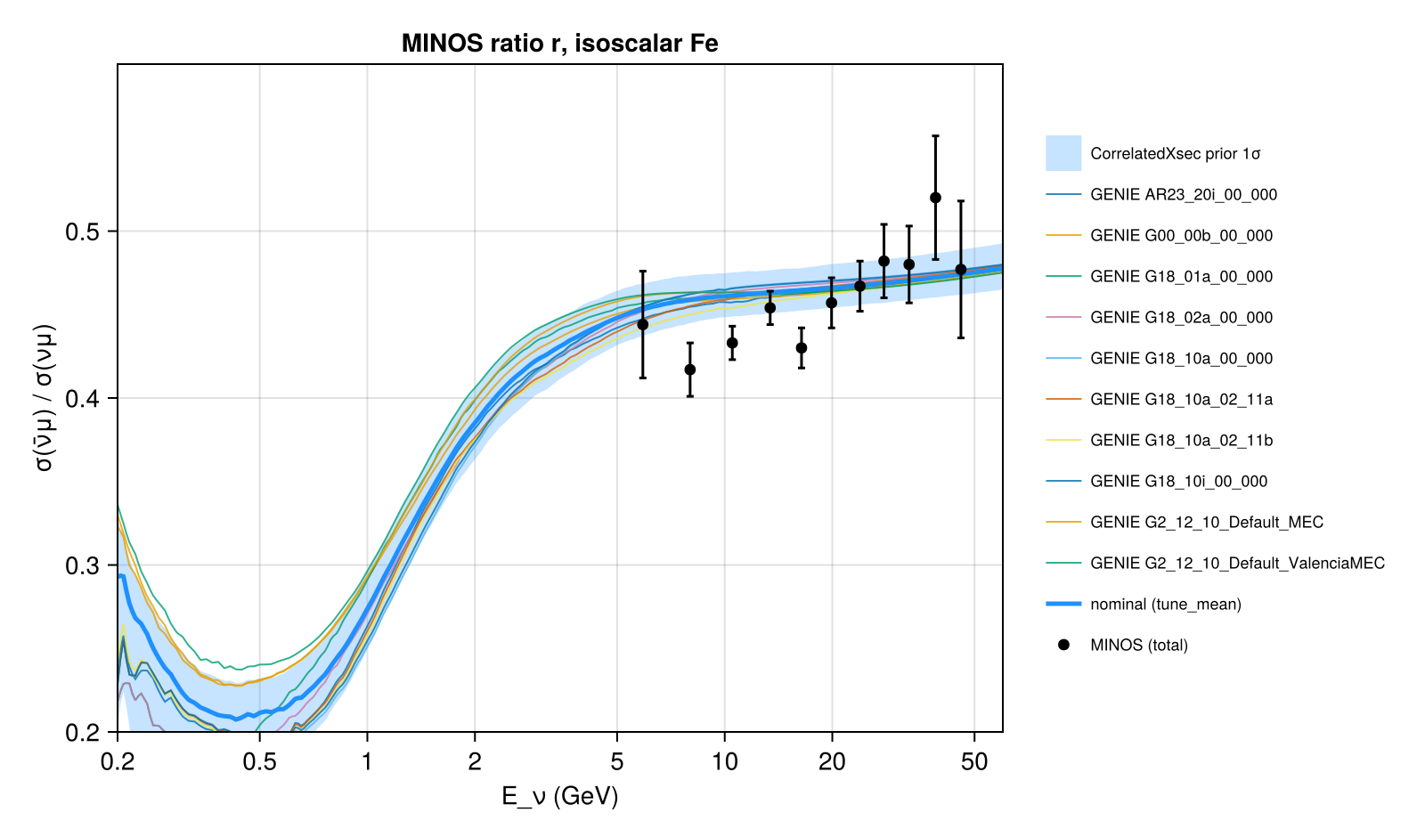
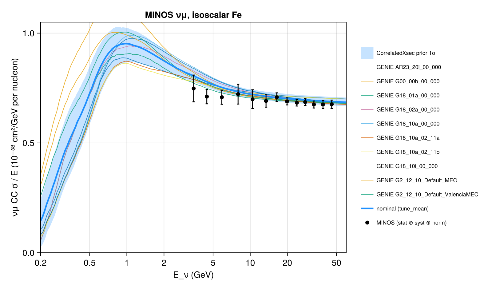
The νμ (3–50 GeV) and ν̄μ (5–50 GeV) inclusive charged-current cross sections per nucleon of isoscalar iron, σ/E, and their ratio r = σ(ν̄)/σ(ν) (the paper's tables, from the arXiv source), compared with the cross sections carried by Newtrinos.jl (module xsec): the ten GENIE tunes of generator_sigma on ⁵⁶Fe, corrected to an isoscalar nucleon with each tune's free proton and neutron cross sections (isoscalar_correction: −2.3 % for ν, +2.1 % for ν̄), and the nominal model of CorrelatedXsec (the mean of the tunes) with its prior 1σ band. The neutrino cross section lies at the upper edge of the data (χ² = 19.5 for 13 bins; 8.0 with the prior band; the tunes give 5–46). The antineutrino cross section between 6 and 16 GeV, and with it the ratio, lies 5–8 % below all tunes (nominal χ² = 16.8/11 for ν̄ and 26.7/11 for r); the prior band of the ratio is ±3 % in this region, including the 3 % ν̄/ν uncertainty of DIS (xsec_nubar_dis_ratio), and with it χ² = 9.2 (ν̄) and 12.8 (r).
Figures
σ(ν̄μ)/σ(νμ) on isoscalar iron: MINOS vs the GENIE tunes and the CorrelatedXsec nominal with its prior 1σ band · Fig. 12 (left)
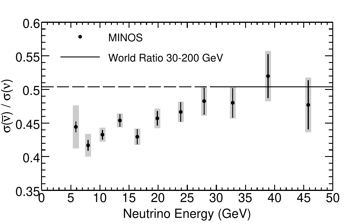
Original figure: MINOS, Phys. Rev. D 81, 072002 (2010), Fig. 12 (left), doi:10.1103/PhysRevD.81.072002. Not our work; shown for comparison, all rights with the authors and publisher.
νμ CC σ/E per isoscalar nucleon of iron · Fig. 10 (left)
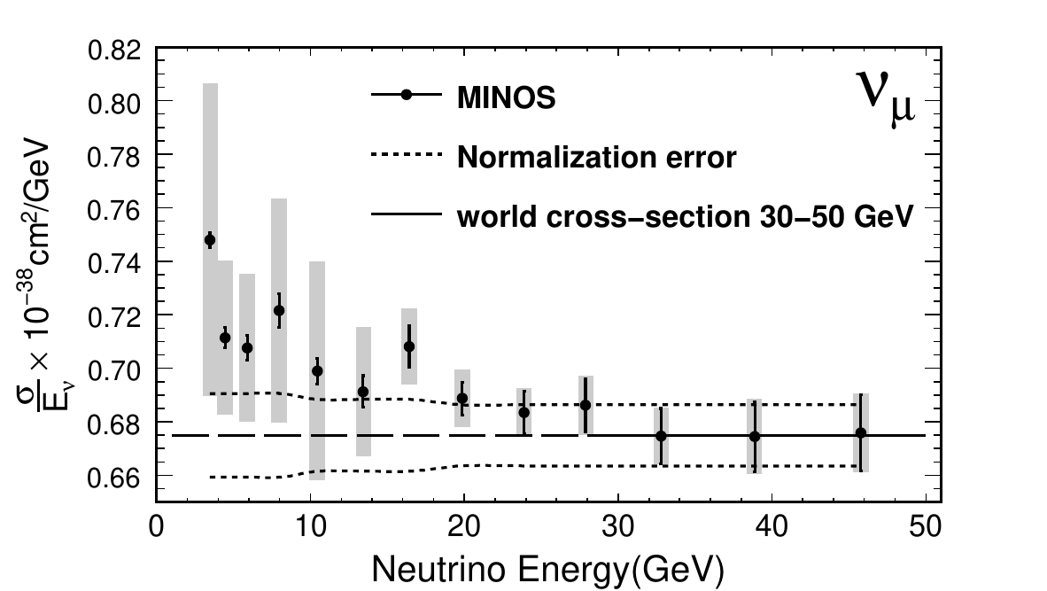
Original figure: MINOS, Phys. Rev. D 81, 072002 (2010), Fig. 10 (left), doi:10.1103/PhysRevD.81.072002. Not our work; shown for comparison, all rights with the authors and publisher.
ν̄μ CC σ/E per isoscalar nucleon of iron · Fig. 10 (right)
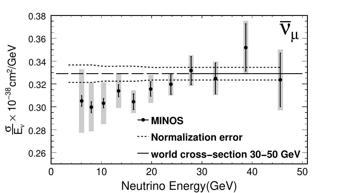
Original figure: MINOS, Phys. Rev. D 81, 072002 (2010), Fig. 10 (right), doi:10.1103/PhysRevD.81.072002. Not our work; shown for comparison, all rights with the authors and publisher.
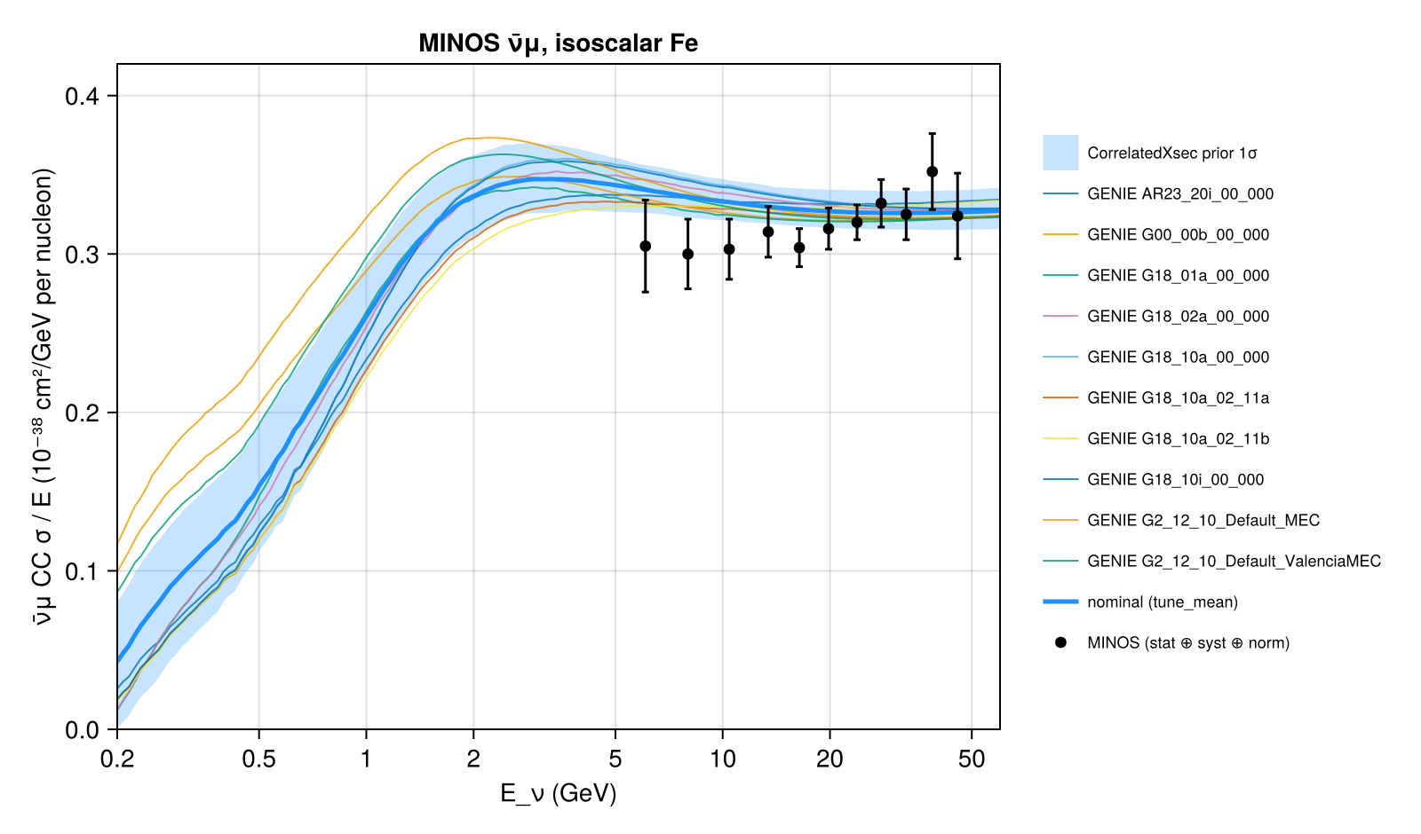
Known limitations
- MINOS normalised the neutrino cross section to the world average (0.675 × 10⁻³⁸ cm²/GeV) above 30 GeV and applied the same constant to the antineutrinos, so absolute normalisations are not tested independently; the ratio r does not depend on it.
- χ² for σ/E uses stat ⊕ syst (the 1.5 % normalisation uncertainty, common to all bins, is left out); for r the total errors. Systematics are partly correlated between bins (no covariance is published). The model is averaged over each σ/E bin (flat in E) and evaluated at the bin-average energy for r.
- The low antineutrino cross section around 10 GeV is a known feature of this measurement; later data (MINERvA's ν̄/ν ratio, a separate entry) can tell whether the shared model needs a ν̄/ν uncertainty in the deep-inelastic region.
- The isoscalar correction is computed from each tune's free-nucleon cross sections; MINOS used its own (NEUGEN3-based) correction.
Reproduce
git clone https://github.com/Newtrinos-org/Newtrinos.jl.git && cd Newtrinos.jl && git checkout 78e71c310b- Download reproduce.jl and the
data/folder of this entry into an empty directory. julia -t 8 --project=/path/to/Newtrinos.jl reproduce.jl
# MINOS νμ and ν̄μ inclusive CC cross sections per nucleon of isoscalar iron, σ/E for 3–50 GeV, and their ratio
# (PRD 81, 072002 (2010); tables from the arXiv:0910.2201 source in data/), compared with the cross sections of
# Newtrinos.jl (module `xsec`): the GENIE tunes (`generator_sigma`, ⁵⁶Fe, corrected to an isoscalar nucleon with each
# tune's free p/n cross sections, `isoscalar_correction`) and the reference model of `CorrelatedXsec` with its prior
# 1σ band (ν, ν̄ and their ratio sampled jointly).
# Run from this directory with the Newtrinos.jl environment at the pinned commit:
#   julia --project=<path to Newtrinos.jl> reproduce.jl
using Newtrinos, CairoMakie, CSV, DataFrames, Printf, Statistics, Random, Distributions

cd(@__DIR__); mkpath("ours"); mkpath("results")
const X = Newtrinos.xsec

d = CSV.read("data/minos_table.csv", DataFrame; comment = "#")
r = CSV.read("data/minos_ratio.csv", DataFrame; comment = "#")
dn, db = d[d.nu .== "nu", :], d[d.nu .== "nubar", :]

tab = X.load_table()
E = 10 .^ range(log10(0.2), log10(60), length = 300)   # down to the threshold region
at(v, e = E) = X.at_energies(tab.E, v, e)
TUNES = Symbol.(sort(tab.tunes))
iso(t, anti, e = E) = at(X.isoscalar_correction(t, 26, 56, :numu, anti), e)
σ_tune(t, anti, e = E) = at(sum(X.generator_sigma(t, :Fe, :numu, anti, :CC)), e) .* iso(t, anti, e)

xs = X.configure(X.CorrelatedXsec())
ref = xs.cfg.reference
sig = Dict(anti => (f = xs.sigma(E; flavour = :numu, anti, current = :CC, target = :Fe); c = iso(ref, anti); p -> f(p) .* c) for anti in (false, true))
# bin averages (flat in E) for the data bins, and the model at the bin-average energies for the ratio
binE(lo, hi) = collect(range(lo, hi, length = 21))
sig_bins(dd, anti) = [(f = xs.sigma(binE(lo, hi); flavour = :numu, anti, current = :CC, target = :Fe); c = iso(ref, anti, binE(lo, hi)); p -> mean(f(p) .* c))
                      for (lo, hi) in zip(dd.E_lo, dd.E_hi)]
bins = (nu = sig_bins(dn, false), nubar = sig_bins(db, true))
sig_r = Dict(anti => (f = xs.sigma(r.E_mean; flavour = :numu, anti, current = :CC, target = :Fe); c = iso(ref, anti, r.E_mean); p -> f(p) .* c) for anti in (false, true))

rng = MersenneTwister(1)
draw() = map(p -> p isa Distribution ? rand(rng, p) : p, xs.priors)
samples = [draw() for _ in 1:500]
q(M, a) = [quantile(filter(!isnan, row), a) for row in eachrow(M)]   # ratios are undefined where a draw has σ = 0
band = Dict(anti => (M = reduce(hcat, [sig[anti](p) for p in samples]); (lo = q(M, 0.16), hi = q(M, 0.84))) for anti in (false, true))
Rs = reduce(hcat, [sig[true](p) ./ sig[false](p) for p in samples])
rband = (lo = q(Rs, 0.16), hi = q(Rs, 0.84))
p0 = xs.params

ticks = ([0.2, 0.5, 1, 2, 5, 10, 20, 50], ["0.2", "0.5", "1", "2", "5", "10", "20", "50"])
function panel_sigma(pos, anti, dd, lab, lims)
    ax = Axis(pos, xscale = log10, xlabel = "E_ν (GeV)", ylabel = "$lab CC σ / E (10⁻³⁸ cm²/GeV per nucleon)",
              title = "MINOS $lab, isoscalar Fe", limits = (0.2, 60, lims...), xticks = ticks)
    band!(ax, E, band[anti].lo, band[anti].hi, color = (:dodgerblue, 0.25), label = "CorrelatedXsec prior 1σ")
    for (i, t) in enumerate(TUNES)
        lines!(ax, E, σ_tune(t, anti), color = (Makie.wong_colors()[mod1(i, 7)], 0.8), linewidth = 1, label = "GENIE $(t)")
    end
    lines!(ax, E, sig[anti](p0), color = :dodgerblue, linewidth = 2.5, label = "nominal ($(ref))")
    errorbars!(ax, dd.E_mean, dd.sigma_over_E, dd.total, color = :black, whiskerwidth = 4)
    scatter!(ax, dd.E_mean, dd.sigma_over_E, color = :black, label = "MINOS (stat ⊕ syst ⊕ norm)")
    ax
end
function panel_ratio(pos)
    ax = Axis(pos, xscale = log10, xlabel = "E_ν (GeV)", ylabel = "σ(ν̄μ) / σ(νμ)", title = "MINOS ratio r, isoscalar Fe",
              limits = (0.2, 60, 0.2, 0.6), xticks = ticks)
    band!(ax, E, rband.lo, rband.hi, color = (:dodgerblue, 0.25), label = "CorrelatedXsec prior 1σ")
    for (i, t) in enumerate(TUNES)
        lines!(ax, E, σ_tune(t, true) ./ σ_tune(t, false), color = (Makie.wong_colors()[mod1(i, 7)], 0.8), linewidth = 1, label = "GENIE $(t)")
    end
    lines!(ax, E, sig[true](p0) ./ sig[false](p0), color = :dodgerblue, linewidth = 2.5, label = "nominal ($(ref))")
    errorbars!(ax, r.E_mean, r.r, r.total, color = :black, whiskerwidth = 4)
    scatter!(ax, r.E_mean, r.r, color = :black, label = "MINOS (total)")
    ax
end
for (name, mk) in (("nu", pos -> panel_sigma(pos, false, dn, "νμ", (0.0, 1.05))),
                   ("nubar", pos -> panel_sigma(pos, true, db, "ν̄μ", (0.0, 0.42))), ("ratio", panel_ratio))
    fig = Figure(size = (800, 470))
    ax = mk(fig[1, 1])
    Legend(fig[1, 2], ax, framevisible = false, labelsize = 9)
    save("ours/$(name).png", fig)
end

# χ²: σ/E with stat ⊕ syst (MINOS normalised ν above 30 GeV to the world average; the normalisation error is common
# to all bins and is left out), and the ratio with its total errors; reference with and without its prior band
chi2(data, err, m, extra = 0) = sum((data .- m) .^ 2 ./ (err .^ 2 .+ extra .^ 2))
err_ss(dd) = sqrt.(dd.stat .^ 2 .+ dd.sys .^ 2)
mref = (nu = [f(p0) for f in bins.nu], nubar = [f(p0) for f in bins.nubar])
msd = (nu = [std([f(p) for p in samples]) for f in bins.nu], nubar = [std([f(p) for p in samples]) for f in bins.nubar])
rref = sig_r[true](p0) ./ sig_r[false](p0)
rsd = [std(col) for col in eachrow(reduce(hcat, [sig_r[true](p) ./ sig_r[false](p) for p in samples]))]
rows = [(model = "$(ref) (nominal)", chi2_nu = chi2(dn.sigma_over_E, err_ss(dn), mref.nu), chi2_nubar = chi2(db.sigma_over_E, err_ss(db), mref.nubar),
         chi2_ratio = chi2(r.r, r.total, rref), chi2_nu_band = chi2(dn.sigma_over_E, err_ss(dn), mref.nu, msd.nu),
         chi2_nubar_band = chi2(db.sigma_over_E, err_ss(db), mref.nubar, msd.nubar), chi2_ratio_band = chi2(r.r, r.total, rref, rsd))]
binavg(t, anti, dd) = [mean(σ_tune(t, anti, binE(lo, hi))) for (lo, hi) in zip(dd.E_lo, dd.E_hi)]
for t in TUNES
    push!(rows, (model = string(t), chi2_nu = chi2(dn.sigma_over_E, err_ss(dn), binavg(t, false, dn)),
                 chi2_nubar = chi2(db.sigma_over_E, err_ss(db), binavg(t, true, db)),
                 chi2_ratio = chi2(r.r, r.total, σ_tune(t, true, r.E_mean) ./ σ_tune(t, false, r.E_mean)),
                 chi2_nu_band = NaN, chi2_nubar_band = NaN, chi2_ratio_band = NaN))
end
out = DataFrame(rows)
out.ndf_nu .= nrow(dn); out.ndf_nubar .= nrow(db); out.ndf_ratio .= nrow(r)
CSV.write("results/chi2.csv", out)
CSV.write("results/ratio.csv", DataFrame(E = r.E_mean, data = r.r, err = r.total, reference = round.(rref, digits = 4), prior_1sigma = round.(rsd, digits = 4)))
show(stdout, out, allrows = true, allcols = true); println()
Provenance
| Newtrinos.jl commit | 78e71c310b (xsec (generator_sigma, isoscalar_correction, CorrelatedXsec)) |
|---|---|
| Run date | 2026-10-12T14:43:11Z |
| Wall time | 1.7 min (4 threads) |
| Julia | 1.12.5 |
| Machine | AMD EPYC 7702P 64-Core Processor, 128 hardware threads, Linux |
| Environment | newtrinos_Manifest.toml · run.toml |
Downloads
CSV files hold one row per scan point: the scanned and profiled parameters
(sin2_theta23, dm2_32 in eV², dcp in rad, nuisance parameters), dchi2 = −2Δ log L
and the log-likelihood. JLD2 files contain the full NewtrinosResult objects.
| File | Size | SHA-256 |
|---|---|---|
| ours/nu.png | 238.3 kB | 5a84faee6bed… |
| ours/nubar.png | 227.9 kB | ca5053dc7a3a… |
| ours/ratio.png | 205.9 kB | a5217f144397… |
| results/chi2.csv | 1.2 kB | ee8284197344… |
| results/ratio.csv | 367 B | 64bc3a1575d9… |