
MiniBooNE · Phys. Rev. D 81, 092005 (2010)
First measurement of the muon neutrino charged current quasielastic double differential cross section
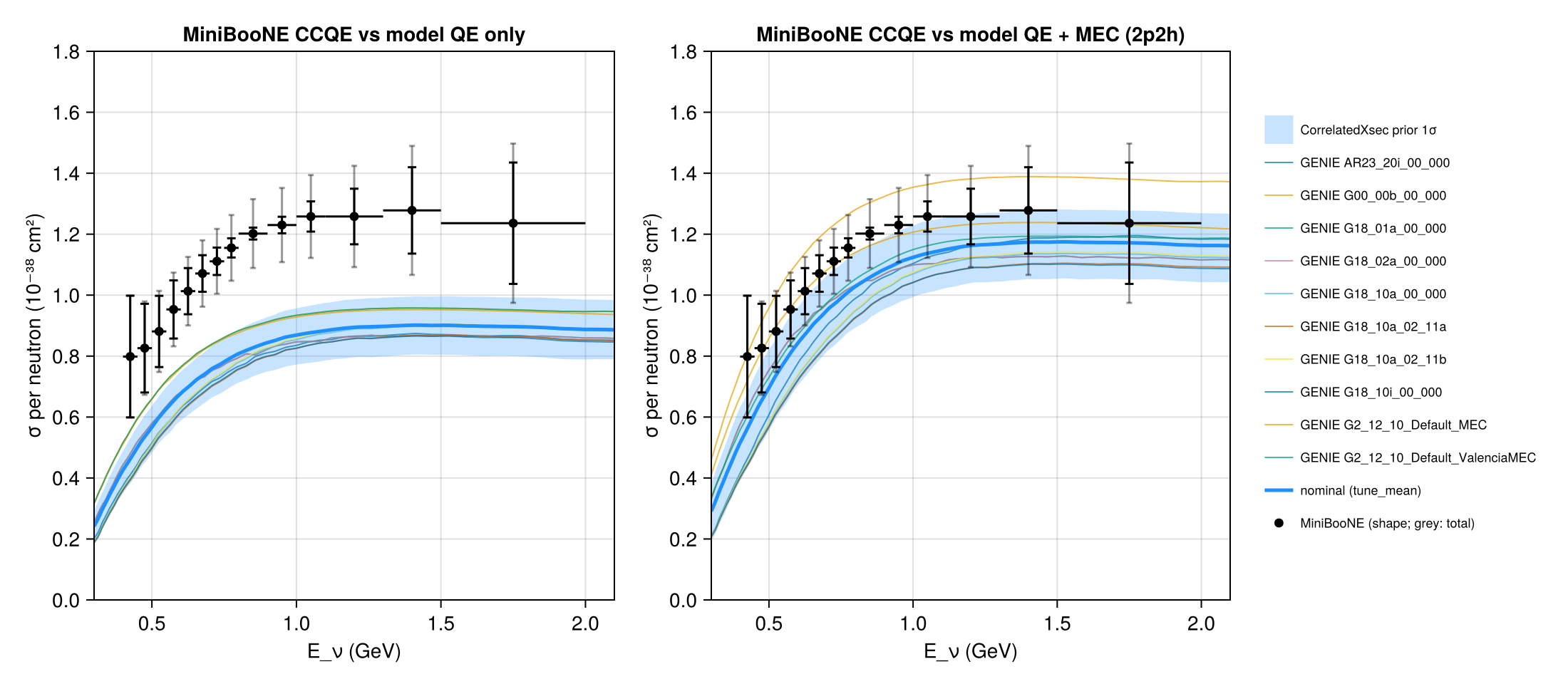
The flux-unfolded νμ CCQE cross section per neutron of carbon (mineral oil), 0.4–2 GeV (Table XI), compared with the cross sections carried by Newtrinos.jl (module xsec): the ten GENIE tunes of generator_sigma on carbon and the nominal model of CorrelatedXsec (the mean of the tunes) with its prior 1σ band, for QE alone and for QE + MEC (2p2h). MiniBooNE's signal is defined by the absence of pions, so it contains 2p2h events: QE alone falls 30–60 % short for all tunes (the origin of MiniBooNE's effective M_A = 1.35 GeV). With MEC the tunes with the empirical MEC model describe the data (G00_00b: χ² = 0.6/14; GENIE 2.12: 10), the Valencia-MEC tunes are 14 % low (G18_01a/02a: 13), G18_10a_02_11a is 33 % low (50.6). The nominal QE + MEC is 16 % below the data (χ² = 16.4; 8.0 with its prior band).
Figures
MiniBooNE νμ CCQE σ per neutron vs the GENIE tunes and the CorrelatedXsec nominal: QE only (left) and QE + MEC (right) · Fig. 15
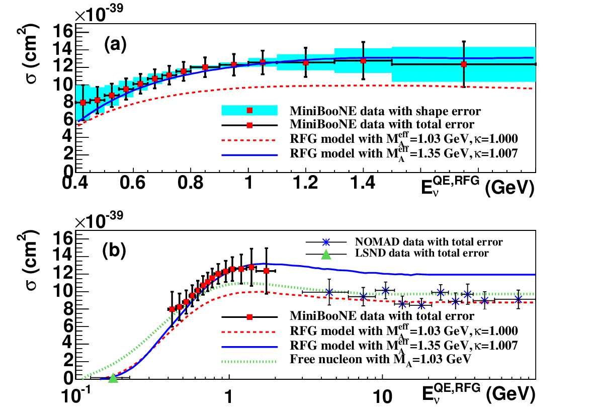
Original figure: MiniBooNE, Phys. Rev. D 81, 092005 (2010), Fig. 15, doi:10.1103/PhysRevD.81.092005. Not our work; shown for comparison, all rights with the authors and publisher.
Known limitations
- Eν is MiniBooNE's unfolded E_ν^{QE,RFG}: the energy is reconstructed from the muon kinematics assuming quasi-elastic scattering on a nucleon at rest, and unfolded with an RFG model. 2p2h events reconstruct at lower energy, so a comparison of the true-energy model cross section with σ(E^QE) is biased at the 10 % level in shape (Nieves et al., Martini et al.); the strong excess over QE alone is nevertheless well established.
- All CC1π⁺ backgrounds, including events whose pion was absorbed in the nucleus, are subtracted with MiniBooNE's tuned NUANCE model. Errors: shape (black) and total including the 10.7 % normalisation (grey); χ² uses the total errors as uncorrelated (no covariance is published for σ(E)).
- Per neutron of carbon: σ per carbon nucleon × 2 (the hydrogen of CH₂ has no neutrons).
- Together with MicroBooNE (argon) this measurement favours the tunes with the larger low-energy cross sections; the nominal (mean of the tunes) lies 16 % below, about one prior standard deviation.
Reproduce
git clone https://github.com/Newtrinos-org/Newtrinos.jl.git && cd Newtrinos.jl && git checkout 78e71c310b- Download reproduce.jl and the
data/folder of this entry into an empty directory. julia -t 8 --project=/path/to/Newtrinos.jl reproduce.jl
# MiniBooNE νμ CCQE cross section per neutron of carbon (mineral oil CH₂), unfolded in Eν, 0.4–2 GeV (PRD 81, 092005
# (2010), Table XI from the arXiv:1002.2680 source, in data/), compared with the cross sections of Newtrinos.jl (module
# `xsec`): the GENIE tunes (`generator_sigma`, carbon; QE only, and QE + MEC) and the reference model of `CorrelatedXsec`
# with its prior 1σ band. MiniBooNE's "CCQE" is defined by the absence of pions (all CC1π⁺ backgrounds, including events
# with an absorbed pion, are subtracted), so 2p2h (MEC) events are part of it: this is the measurement that led to an
# effective axial mass of 1.35 GeV in a QE-only model.
# Run from this directory with the Newtrinos.jl environment at the pinned commit:
#   julia --project=<path to Newtrinos.jl> reproduce.jl
using Newtrinos, CairoMakie, CSV, DataFrames, Printf, Statistics, Random, Distributions

cd(@__DIR__); mkpath("ours"); mkpath("results")
const X = Newtrinos.xsec

D = CSV.read("data/miniboone_nu.csv", DataFrame; comment = "#")
Ec = (D.E_lo .+ D.E_hi) ./ 2

tab = X.load_table()
E = collect(range(0.2, 2.2, length = 300))
at(v, e = E) = X.at_energies(tab.E, v, e)
TUNES = Symbol.(sort(tab.tunes))
# per neutron of carbon = σ per carbon nucleon × 12/6
σ_tune(t, procs, e = E) = at(sum(getfield(X.generator_sigma(t, :C, :numu, false, :CC), p) for p in procs), e) .* e .* 2

xs = X.configure(X.CorrelatedXsec())
ref = xs.cfg.reference
sigma(procs, e = E) = (f = xs.sigma(e; flavour = :numu, anti = false, current = :CC, target = :C, process = procs); p -> f(p) .* e .* 2)
rng = MersenneTwister(1)
draw() = map(p -> p isa Distribution ? rand(rng, p) : p, xs.priors)
samples = [draw() for _ in 1:500]
p0 = xs.params
q(M, a) = [quantile(r, a) for r in eachrow(M)]

fig = Figure(size = (1100, 480))
for (k, (procs, lab)) in enumerate((((:QE,), "QE only"), ((:QE, :MEC), "QE + MEC (2p2h)")))
    ax = Axis(fig[1, k], xlabel = "E_ν (GeV)", ylabel = "σ per neutron (10⁻³⁸ cm²)", title = "MiniBooNE CCQE vs model $(lab)",
              limits = (0.3, 2.1, 0, 1.8))
    f = sigma(procs)
    M = reduce(hcat, [f(p) for p in samples])
    band!(ax, E, q(M, 0.16), q(M, 0.84), color = (:dodgerblue, 0.25), label = "CorrelatedXsec prior 1σ")
    for (i, t) in enumerate(TUNES)
        lines!(ax, E, σ_tune(t, procs), color = (Makie.wong_colors()[mod1(i, 7)], 0.7), linewidth = 1, label = "GENIE $(t)")
    end
    lines!(ax, E, f(p0), color = :dodgerblue, linewidth = 2.5, label = "nominal ($(ref))")
    errorbars!(ax, Ec, D.sigma_ccqe, D.err_total, color = (:black, 0.4), whiskerwidth = 4)
    errorbars!(ax, Ec, D.sigma_ccqe, D.err_shape, color = :black, whiskerwidth = 6)
    errorbars!(ax, Ec, D.sigma_ccqe, Ec .- D.E_lo, D.E_hi .- Ec, direction = :x, color = :black)
    scatter!(ax, Ec, D.sigma_ccqe, color = :black, label = "MiniBooNE (shape; grey: total)")
    k == 2 && Legend(fig[1, 3], ax, framevisible = false, labelsize = 9)
end
save("ours/sigma.png", fig)

# χ² with the total errors (uncorrelated; the 10.7 % normalisation is common to all bins) and the mean data/model ratio,
# for the model averaged flat over each bin
binavg(f) = [mean(f(collect(range(lo, hi, length = 11)))) for (lo, hi) in zip(D.E_lo, D.E_hi)]
chi2(m, extra = 0) = sum((D.sigma_ccqe .- m) .^ 2 ./ (D.err_total .^ 2 .+ extra .^ 2))
rows = []
for (procs, lab) in (((:QE,), "QE"), ((:QE, :MEC), "QE+MEC"))
    fb = [sigma(procs, collect(range(lo, hi, length = 11))) for (lo, hi) in zip(D.E_lo, D.E_hi)]
    m0 = [mean(f(p0)) for f in fb]
    sd = vec(std(reduce(hcat, [[mean(f(p)) for f in fb] for p in samples]), dims = 2))
    push!(rows, (model = "$(ref) (nominal)", process = lab, chi2 = chi2(m0), chi2_with_prior = chi2(m0, sd), data_over_model = mean(D.sigma_ccqe ./ m0)))
    for t in TUNES
        m = binavg(e -> σ_tune(t, procs, e))
        push!(rows, (model = string(t), process = lab, chi2 = chi2(m), chi2_with_prior = NaN, data_over_model = mean(D.sigma_ccqe ./ m)))
    end
end
out = DataFrame(rows); out.ndf .= nrow(D)
out.chi2 = round.(out.chi2, digits = 2); out.data_over_model = round.(out.data_over_model, digits = 3)
CSV.write("results/chi2.csv", out)
show(stdout, out, allrows = true); println()
Provenance
| Newtrinos.jl commit | 78e71c310b (xsec (generator_sigma, CorrelatedXsec)) |
|---|---|
| Run date | 2026-10-12T12:27:10Z |
| Wall time | 1.4 min (4 threads) |
| Julia | 1.12.5 |
| Machine | AMD EPYC 7702P 64-Core Processor, 128 hardware threads, Linux |
| Environment | newtrinos_Manifest.toml · run.toml |
Downloads
CSV files hold one row per scan point: the scanned and profiled parameters
(sin2_theta23, dm2_32 in eV², dcp in rad, nuisance parameters), dchi2 = −2Δ log L
and the log-likelihood. JLD2 files contain the full NewtrinosResult objects.
| File | Size | SHA-256 |
|---|---|---|
| ours/sigma.png | 284.6 kB | 1569638d6c4a… |
| results/chi2.csv | 994 B | 31bb9f1efb8d… |