
J. Conrad, A. de Gouvêa, S. Shalgar, J. Spitz · Phys. Rev. D 82, 093012 (2010)
Atmospheric tau neutrinos in a multi-kiloton liquid argon detector
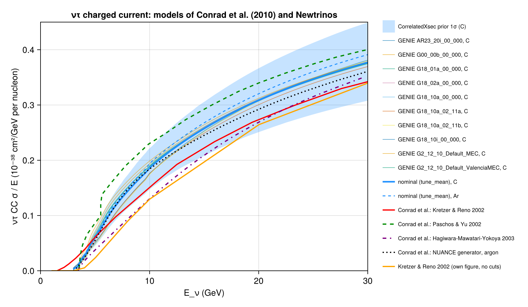
The ντ charged-current cross section, which has a kinematic threshold (≈ 3.5 GeV) and is suppressed by the τ mass up \
to high energies, compared between the models of Conrad et al. (Kretzer–Reno, Paschos–Yu, Hagiwara–Mawatari–Yokoya on \
an isoscalar target and NUANCE on argon; vector-digitised from the arXiv figure), the NLO deep-inelastic calculations of \
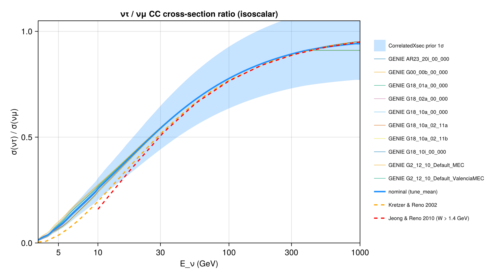
Kretzer & Reno (2002) and Jeong & Reno (2010) for σ(ντ)/σ(νμ), and the cross sections carried by Newtrinos.jl (module \
xsec): the ten GENIE tunes of generator_sigma (carbon and argon) and the nominal model of CorrelatedXsec (the mean \
of the tunes) with its prior 1σ band. The GENIE tunes agree with each other to a few % and lie between the models of the \
paper; fitted with the paper's threshold parametrisation σ/E = (1 − exp(−a √(E − b))) × 10⁻³⁸ cm²/GeV on 4–30 GeV, the \
nominal gives a = 0.094, b = 4.7 GeV (carbon), as NUANCE (0.089, 4.7 GeV) in the paper's table (Kretzer–Reno 0.080, \
5.6 GeV; Paschos–Yu 0.105, 4.1 GeV). The ratio σ(ντ)/σ(νμ) agrees with Jeong–Reno and Kretzer–Reno above 30 GeV to \
1–2 % and is up to 30 % higher at 10 GeV, where the nuclear QE and resonance contributions, absent in their DIS \
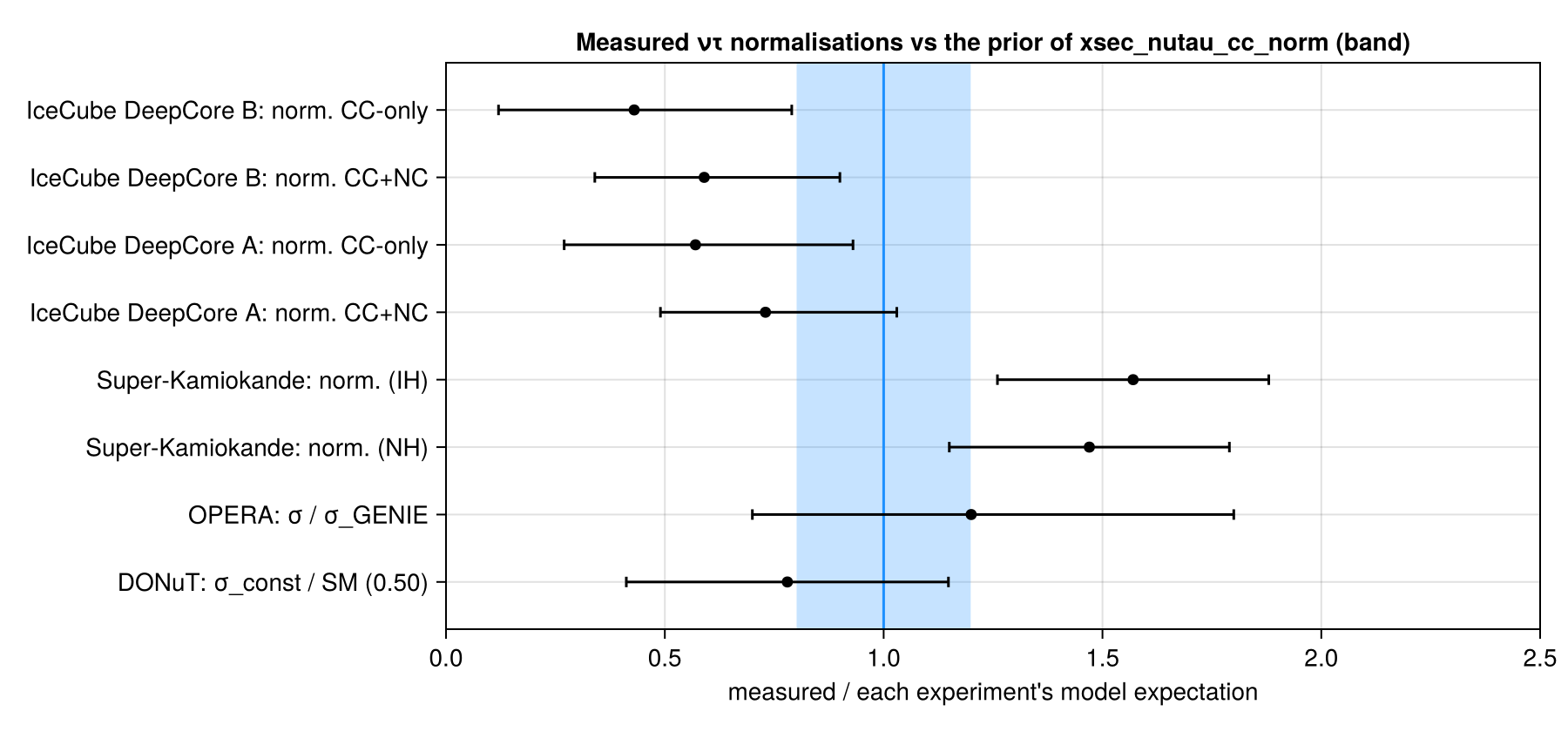
calculation, matter. The measured ντ normalisations (relative to each experiment's model) scatter around 1: Super-K \
1.47 ± 0.32, IceCube DeepCore 0.57–0.73 (CC: 0.57 +0.36/−0.30), OPERA 1.2 +0.6/−0.5, DONuT 0.78 ± 0.37.
Figures
ντ CC σ/E: the models of Conrad et al. and Kretzer–Reno vs the GENIE tunes and the CorrelatedXsec nominal with its prior 1σ band · Fig. 5
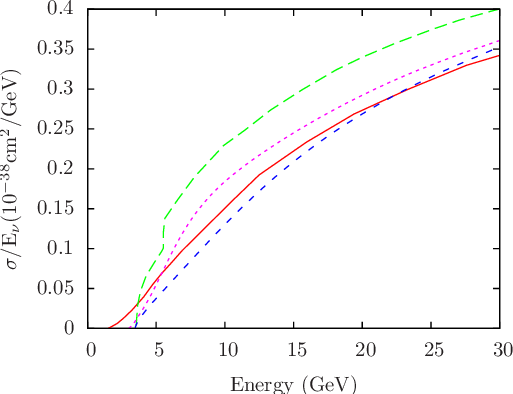
Original figure: J. Conrad, A. de Gouvêa, S. Shalgar, J. Spitz, Phys. Rev. D 82, 093012 (2010), Fig. 5, doi:10.1103/PhysRevD.82.093012. Not our work; shown for comparison, all rights with the authors and publisher.
σ(ντ)/σ(νμ): Kretzer–Reno and Jeong–Reno vs the GENIE tunes and the CorrelatedXsec nominal · Jeong & Reno 2010, Fig. 2
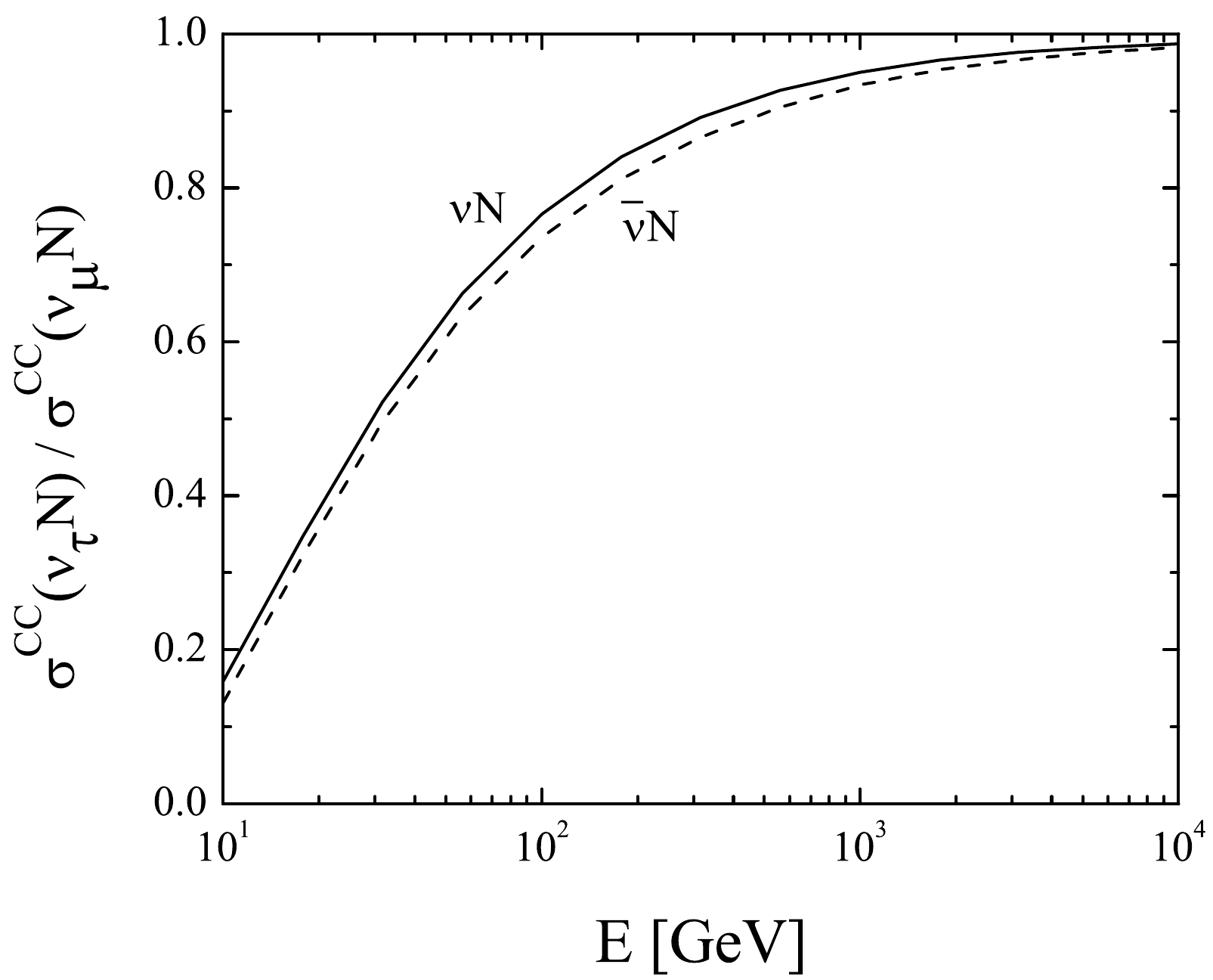
Original figure: J. Conrad, A. de Gouvêa, S. Shalgar, J. Spitz, Phys. Rev. D 82, 093012 (2010), Jeong & Reno 2010, Fig. 2, doi:10.1103/PhysRevD.82.093012. Not our work; shown for comparison, all rights with the authors and publisher.
Measured ντ normalisations (DONuT, OPERA, Super-K, IceCube DeepCore) and the prior of the shared ντ normalisation ·
no figure
Known limitations
- The models in Conrad et al.'s figure are digitised from the vector graphics; their 'Kretzer et al.' curve starts below the free-nucleon threshold and is ~25 % above Kretzer & Reno's own curve at 10 GeV (0.16 vs 0.13), so Kretzer & Reno's own (no-cut) curve is shown as well. The NLO calculations are DIS only (Jeong–Reno with W > 1.4 GeV), so they lack the quasi-elastic and resonance contributions near threshold.
- The prior band includes the 20 % ντ normalisation (xsec_nutau_cc_norm), which is energy independent; at high energies, where σ(ντ)/σ(νμ) → 1 is well known, it overstates the uncertainty, near threshold it is the dominant model uncertainty (τ-mass corrections, structure functions F4/F5, nuclear effects).
- The measured normalisations refer to different models (Super-K: NEUT; DeepCore: GENIE 2.8.6; OPERA: GENIE 2.6; DONuT: σ_const relative to the Standard-Model value 0.50 × 10⁻³⁸ cm²/GeV) and different energy ranges, and they are correlated with oscillation parameters and flux uncertainties in the fits; they are not a direct cross-section measurement except for DONuT and OPERA. A fit of xsec_nutau_cc_norm with Super-K and DeepCore and the shared model is on the roadmap.
- GENIE 2.12 splines end at 400 GeV; above, σ/E is held constant, which flattens its ratio.
Reproduce
git clone https://github.com/Newtrinos-org/Newtrinos.jl.git && cd Newtrinos.jl && git checkout 78e71c310b- Download reproduce.jl and the
data/folder of this entry into an empty directory. julia -t 8 --project=/path/to/Newtrinos.jl reproduce.jl
# ντ charged-current cross sections: the models compared by Conrad, de Gouvêa, Shalgar & Spitz, PRD 82, 093012 (2010)
# (Kretzer–Reno, Paschos–Yu, Hagiwara–Mawatari–Yokoya on an isoscalar target, NUANCE on argon; vector-digitised from the
# arXiv source figure), the NLO DIS calculations of Kretzer & Reno (2002) and Jeong & Reno (2010) for σ(ντ)/σ(νμ), and
# the measured ντ normalisations (DONuT, OPERA, Super-K, IceCube DeepCore), compared with the ντ cross sections of
# Newtrinos.jl (module `xsec`): the GENIE tunes (`generator_sigma`, carbon = isoscalar, and argon) and the nominal model of
# `CorrelatedXsec` (the mean of the tunes) with its prior 1σ band, which includes the ντ normalisation (20 %).
# Run from this directory with the Newtrinos.jl environment at the pinned commit:
#   julia --project=<path to Newtrinos.jl> reproduce.jl
using Newtrinos, CairoMakie, CSV, DataFrames, Printf, Statistics, Random, Distributions

cd(@__DIR__); mkpath("ours"); mkpath("results")
const X = Newtrinos.xsec

S = CSV.read("data/sigma_nutau.csv", DataFrame; normalizenames = true)
R = CSV.read("data/ratio_tau_mu.csv", DataFrame)
M = CSV.read("data/measurements.csv", DataFrame)
P = CSV.read("data/conrad2010_models_param_fluxavg.csv", DataFrame)

tab = X.load_table()
at(v, e) = X.at_energies(tab.E, v, e)
TUNES = Symbol.(sort(tab.tunes))
σE(t, target, flavour, anti, e) = at(sum(X.generator_sigma(t, target, flavour, anti, :CC)), e)

xs = X.configure(X.CorrelatedXsec())
ref = xs.cfg.reference
rng = MersenneTwister(1)
draw() = map(p -> p isa Distribution ? rand(rng, p) : p, xs.priors)
samples = [draw() for _ in 1:500]
p0 = xs.params
q(Mx, a) = [quantile(r, a) for r in eachrow(Mx)]
tunecol(i) = (Makie.wong_colors()[mod1(i, 7)], 0.6)

# --- σ/E for ντ, 0–30 GeV (Conrad et al. figure)
E = collect(range(3.0, 30.0, length = 300))
fτ = Dict(tg => xs.sigma(E; flavour = :nutau, anti = false, current = :CC, target = tg) for tg in (:C, :Ar))
fig = Figure(size = (860, 500))
ax = Axis(fig[1, 1], xlabel = "E_ν (GeV)", ylabel = "ντ CC σ / E (10⁻³⁸ cm²/GeV per nucleon)", limits = (0, 30, 0, 0.45),
          title = "ντ charged current: models of Conrad et al. (2010) and Newtrinos")
Mb = reduce(hcat, [fτ[:C](p) for p in samples])
band!(ax, E, q(Mb, 0.16), q(Mb, 0.84), color = (:dodgerblue, 0.25), label = "CorrelatedXsec prior 1σ (C)")
for (i, t) in enumerate(TUNES)
    lines!(ax, E, σE(t, :C, :nutau, false, E), color = tunecol(i), linewidth = 1, label = "GENIE $(t), C")
end
lines!(ax, E, fτ[:C](p0), color = :dodgerblue, linewidth = 2.5, label = "nominal ($(ref)), C")
lines!(ax, E, fτ[:Ar](p0), color = :dodgerblue, linewidth = 1.5, linestyle = :dash, label = "nominal ($(ref)), Ar")
cs = S[S.source .== "Conrad_deGouvea_Shalgar_Spitz_2010_Fig", :]
for (m, col, ls) in zip(unique(cs.model), (:red, :green4, :purple, :black), (:solid, :dash, :dashdot, :dot))
    d = cs[cs.model .== m, :]
    lines!(ax, d.E_GeV, d.sigma_over_E_1e_38cm2_per_GeV, color = col, linestyle = ls, linewidth = 2, label = "Conrad et al.: " * replace(m, " (as plotted by Conrad et al.)" => ""))
end
kr = S[(S.source .== "Kretzer_Reno_2002_Fig6") .& (S.neutrino .== "nu_tau") .& occursin.("inclusive", S.process), :]
lines!(ax, kr.E_GeV, kr.sigma_over_E_1e_38cm2_per_GeV, color = :orange, linewidth = 2, label = "Kretzer & Reno 2002 (own figure, no cuts)")
Legend(fig[1, 2], ax, framevisible = false, labelsize = 9)
save("ours/sigma_over_E.png", fig)

# --- σ(ντ)/σ(νμ), 3–1000 GeV
E2 = 10 .^ range(log10(3.5), 3, length = 300)
fμ = xs.sigma(E2; flavour = :numu, anti = false, current = :CC, target = :C)
fτ2 = xs.sigma(E2; flavour = :nutau, anti = false, current = :CC, target = :C)
Mr = reduce(hcat, [fτ2(p) ./ fμ(p) for p in samples])
fig = Figure(size = (860, 480))
ax = Axis(fig[1, 1], xscale = log10, xlabel = "E_ν (GeV)", ylabel = "σ(ντ) / σ(νμ)", limits = (3.5, 1000, 0, 1.05),
          xticks = ([5, 10, 30, 100, 300, 1000], ["5", "10", "30", "100", "300", "1000"]), title = "ντ / νμ CC cross-section ratio (isoscalar)")
band!(ax, E2, q(Mr, 0.16), q(Mr, 0.84), color = (:dodgerblue, 0.25), label = "CorrelatedXsec prior 1σ")
for (i, t) in enumerate(TUNES)
    lines!(ax, E2, σE(t, :C, :nutau, false, E2) ./ σE(t, :C, :numu, false, E2), color = tunecol(i), linewidth = 1, label = "GENIE $(t)")
end
lines!(ax, E2, fτ2(p0) ./ fμ(p0), color = :dodgerblue, linewidth = 2.5, label = "nominal ($(ref))")
for (src, col, lab) in (("Kretzer_Reno_2002_Fig6_lower", :orange, "Kretzer & Reno 2002"), ("Jeong_Reno_2010_Fig2", :red, "Jeong & Reno 2010 (W > 1.4 GeV)"))
    d = R[(R.source .== src) .& startswith.(R.neutrino, "nu ("), :]
    lines!(ax, d.E_GeV, d.ratio_sigma_tau_over_sigma_mu, color = col, linewidth = 2, linestyle = :dash, label = lab)
end
Legend(fig[1, 2], ax, framevisible = false, labelsize = 9)
save("ours/ratio_tau_mu.png", fig)

# --- the threshold parametrisation of Conrad et al., σ/E = (1 − exp(−a √(E − b))) × 10⁻³⁸ cm²/GeV, fitted on 4–30 GeV
Efit = collect(range(4.0, 30.0, length = 100))
function fitab(y)
    best = (Inf, 0.0, 0.0)
    for a in 0.05:0.0005:0.15, b in 2.5:0.02:7.0
        m = 1 .- exp.(-a .* sqrt.(max.(Efit .- b, 0)))
        c = sum((y .- m) .^ 2)
        c < best[1] && (best = (c, a, b))
    end
    best[2], best[3]
end
a, b = fitab(xs.sigma(Efit; flavour = :nutau, anti = false, current = :CC, target = :C)(p0))
rows = [(model = "nominal ($(ref)), C", a = a, b = b)]
for t in TUNES
    a, b = fitab(σE(t, :C, :nutau, false, Efit)); push!(rows, (model = "GENIE $(t), C", a = a, b = b))
end
a, b = fitab(xs.sigma(Efit; flavour = :nutau, anti = false, current = :CC, target = :Ar)(p0)); push!(rows, (model = "nominal ($(ref)), Ar", a = a, b = b))
for r in eachrow(P)
    push!(rows, (model = "Conrad et al.: " * r.model, a = r.a, b = r.b_GeV))
end
ab = DataFrame(rows)
CSV.write("results/threshold_parametrisation.csv", ab)
show(stdout, ab, allrows = true); println()

# --- measured ντ normalisations vs the prior of the nominal model's ντ normalisation (xsec_nutau_cc_norm)
sel = [r for r in eachrow(M) if occursin("normalisation", r.quantity) || occursin("ratio <sigma>", r.quantity) || startswith(r.quantity, "sigma_const") && !occursin("superseded", r.experiment)]
short(q) = startswith(q, "sigma_const") ? "σ_const / SM (0.50)" : q == "ratio <sigma>_meas/<sigma>_GENIE" ? "σ / σ_GENIE" :
           replace(q, "nu_tau normalisation" => "norm.", "tau normalisation" => "norm.")
labs = ["$(replace(r.experiment, " (Analysis A)" => " A", " (Analysis B; confirmatory)" => " B")): $(short(r.quantity))" for r in sel]
vals = [r.quantity |> s -> startswith(s, "sigma_const") ? r.value / 0.50 : r.value for r in sel]   # DONuT: σ_const / SM value 0.50
eu = [startswith(r.quantity, "sigma_const") ? r.err_up / 0.50 : r.err_up for r in sel]
ed = [startswith(r.quantity, "sigma_const") ? r.err_down / 0.50 : r.err_down for r in sel]
fig = Figure(size = (900, 420))
ax = Axis(fig[1, 1], xlabel = "measured / each experiment's model expectation", yticks = (1:length(sel), labs), limits = (0, 2.5, 0.3, length(sel) + 0.7),
          title = "Measured ντ normalisations vs the prior of xsec_nutau_cc_norm (band)")
nτ = xs.priors.xsec_nutau_cc_norm
vspan!(ax, [quantile(nτ, 0.16)], [quantile(nτ, 0.84)], color = (:dodgerblue, 0.25))
vlines!(ax, [1.0], color = :dodgerblue)
errorbars!(ax, vals, 1:length(sel), ed, eu, direction = :x, color = :black, whiskerwidth = 6)
scatter!(ax, vals, 1:length(sel), color = :black)
save("ours/measurements.png", fig)
Provenance
| Newtrinos.jl commit | 78e71c310b (xsec (generator_sigma, CorrelatedXsec)) |
|---|---|
| Run date | 2026-10-12T12:11:01Z |
| Wall time | 1.6 min (4 threads) |
| Julia | 1.12.5 |
| Machine | AMD EPYC 7702P 64-Core Processor, 128 hardware threads, Linux |
| Environment | newtrinos_Manifest.toml · run.toml |
Downloads
CSV files hold one row per scan point: the scanned and profiled parameters
(sin2_theta23, dm2_32 in eV², dcp in rad, nuisance parameters), dchi2 = −2Δ log L
and the log-likelihood. JLD2 files contain the full NewtrinosResult objects.
| File | Size | SHA-256 |
|---|---|---|
| ours/measurements.png | 143.1 kB | 3e9fa0495fa9… |
| ours/ratio_tau_mu.png | 180.5 kB | af4142c98c1e… |
| ours/sigma_over_E.png | 300.3 kB | 6876f2b7e37a… |
| results/threshold_parametrisation.csv | 786 B | 7e0346a1e881… |