
KamLAND · Phys. Rev. D 88, 033001 (2013)
Reactor On-Off Antineutrino Measurement with KamLAND
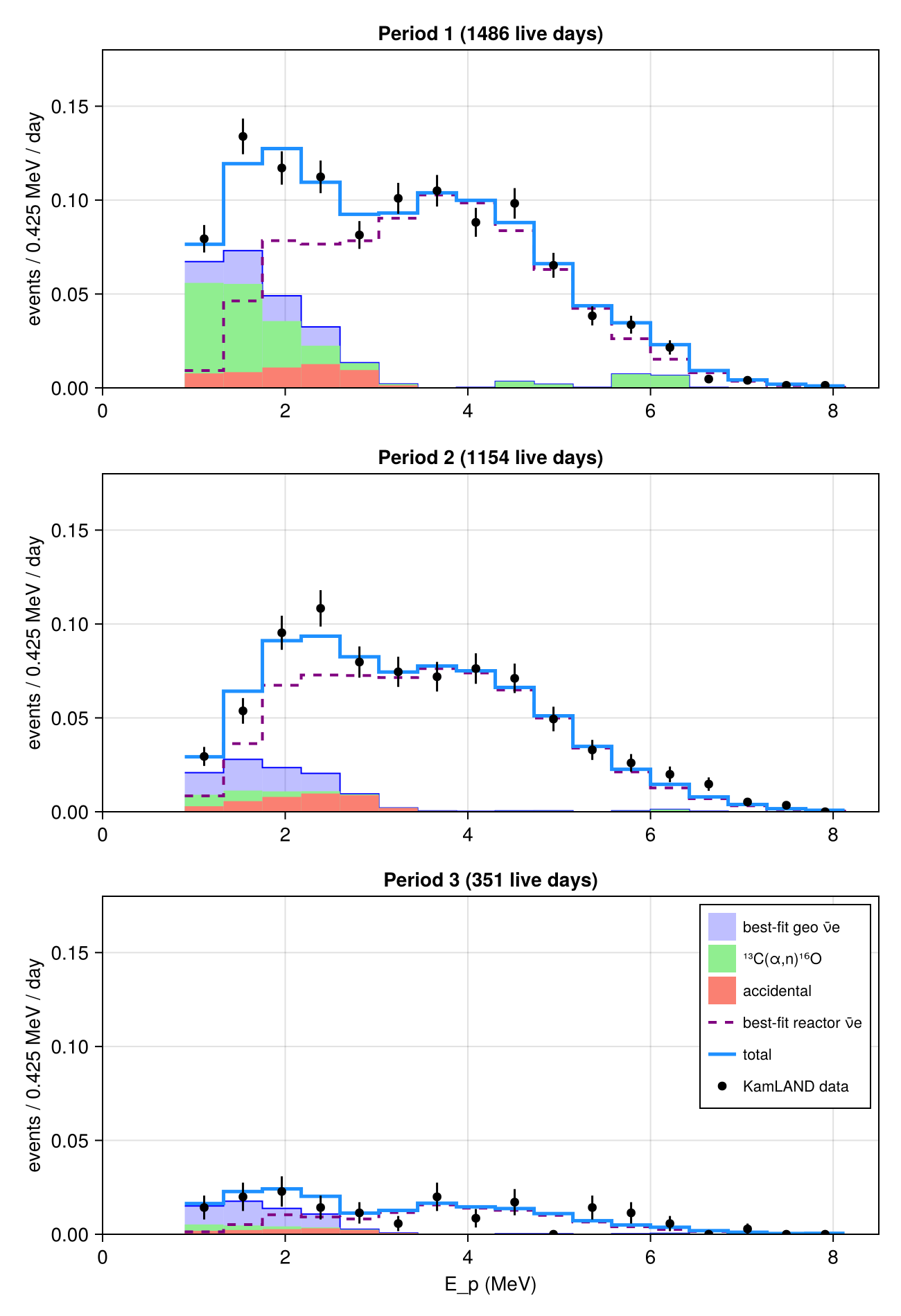
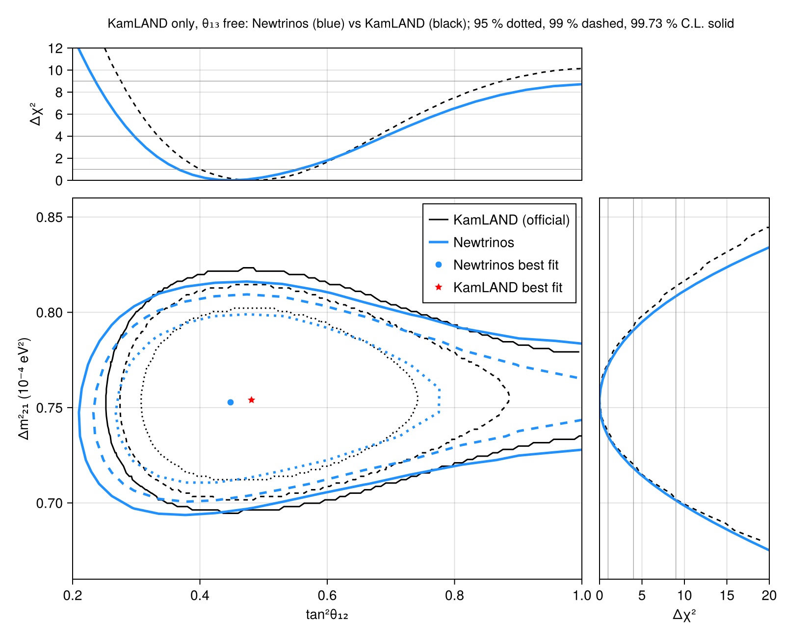
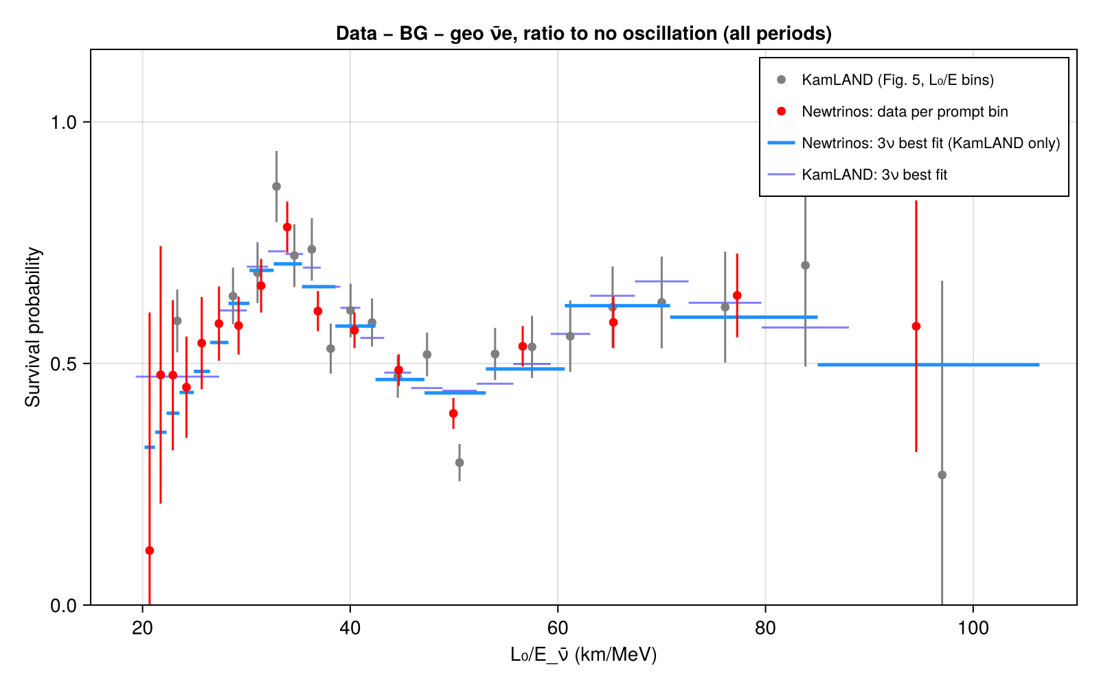
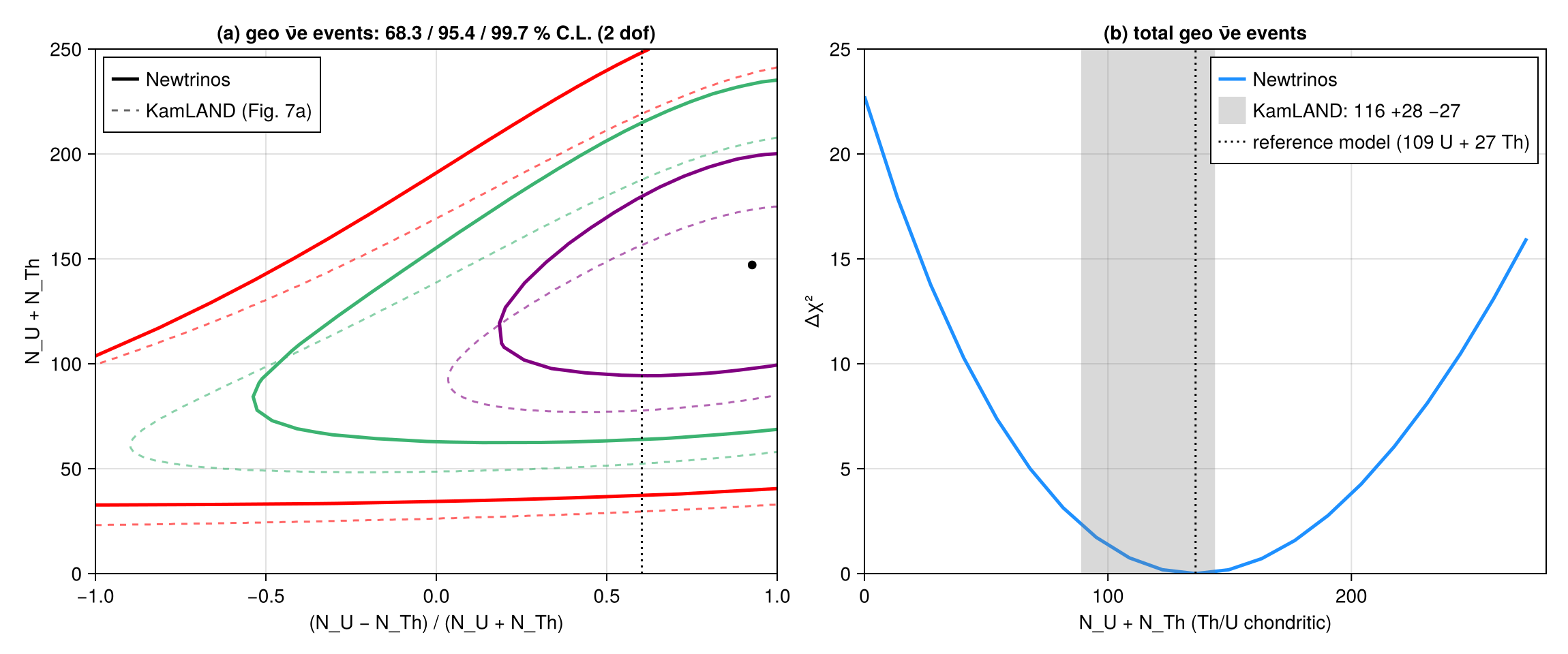
KamLAND's 2002–2012 data in the three data-taking periods of the paper (before and after the scintillator purification, and the post-Fukushima reactor-off period), with the reactor ν̄e prediction computed from first principles: the thermal power histories of all Japanese and Korean power reactors (IAEA PRIS), the site baselines, Huber–Mueller spectra anchored to Bugey-4, the IBD cross section, 3ν oscillations with matter effects, energy resolution and the selection efficiency of each period; KamLAND's systematics (reactor rate, energy scale, ¹³C(α,n), ⁹Li) and free geo-ν̄e U and Th. Nothing is tuned to KamLAND's fit: the no-oscillation expectation, 3631 events, agrees with KamLAND's 3564 ± 145, and the spectral shape with KamLAND's published expectation for the 2002–2009 data (χ² 1.9 for 17 bins). The KamLAND-only fit with θ₁₃ free gives Δm²₂₁ = 7.55 +0.17 −0.20 ×10⁻⁵ eV² and tan²θ₁₂ = 0.451 +0.103 −0.085 (KamLAND: 7.54 +0.19 −0.18, 0.481 +0.092 −0.080). Also shown: the ratio to no oscillation vs L₀/E (Fig. 5) and the geo-ν̄e event numbers (Fig. 7): with the oscillation parameters at the paper's solar + KamLAND + θ₁₃ values and the chondritic Th/U ratio, Newtrinos finds N_U + N_Th = 136 +32 −31 (KamLAND: 116 +28 −27); the (N_U, N_Th) regions have KamLAND's shape, shifted up by about 15–20 events.
Figures
Prompt energy spectra per data-taking period with the best-fit contributions (KamLAND only) · Fig. 3
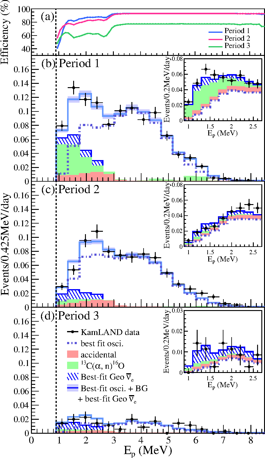
Original figure: KamLAND, Phys. Rev. D 88, 033001 (2013), Fig. 3, doi:10.1103/PhysRevD.88.033001. Not our work; shown for comparison, all rights with the authors and publisher.
KamLAND-only allowed regions in (tan²θ₁₂, Δm²₂₁), θ₁₃ free, 95 %, 99 %, 99.73 % C.L., with Δχ² profiles; Newtrinos (blue) overlaid on KamLAND (black, from the vector graphics of the paper figure) · Fig. 4(a)
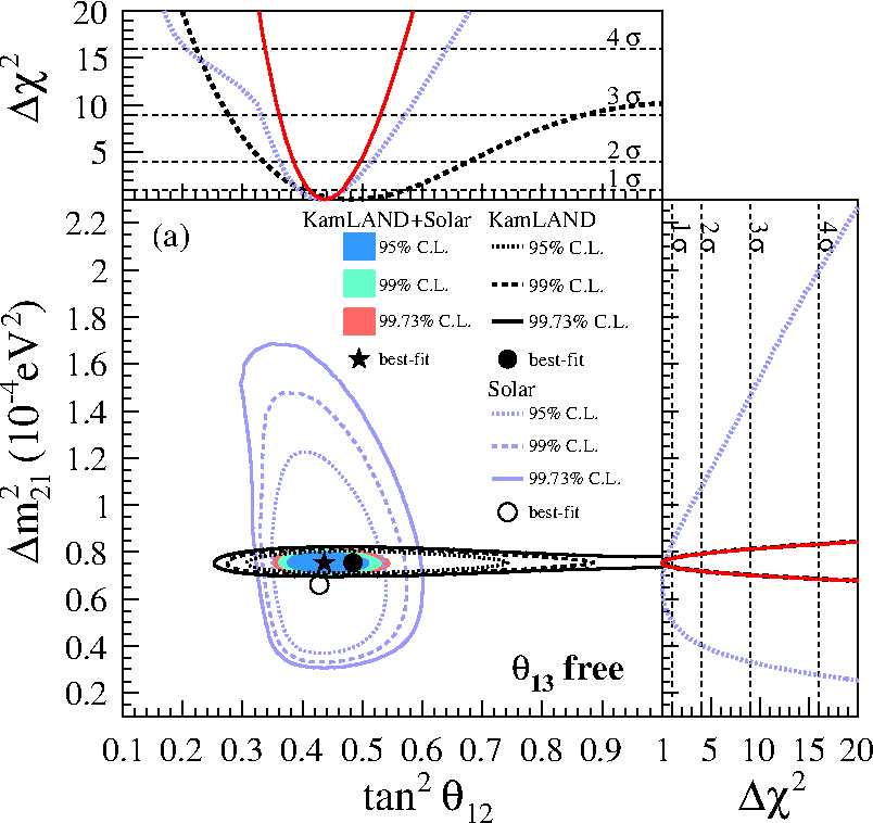
Original figure: KamLAND, Phys. Rev. D 88, 033001 (2013), Fig. 4(a), doi:10.1103/PhysRevD.88.033001. Not our work; shown for comparison, all rights with the authors and publisher.
Ratio of the observed spectrum (minus backgrounds and geo ν̄e) to no oscillation vs L₀/E, all periods · Fig. 5
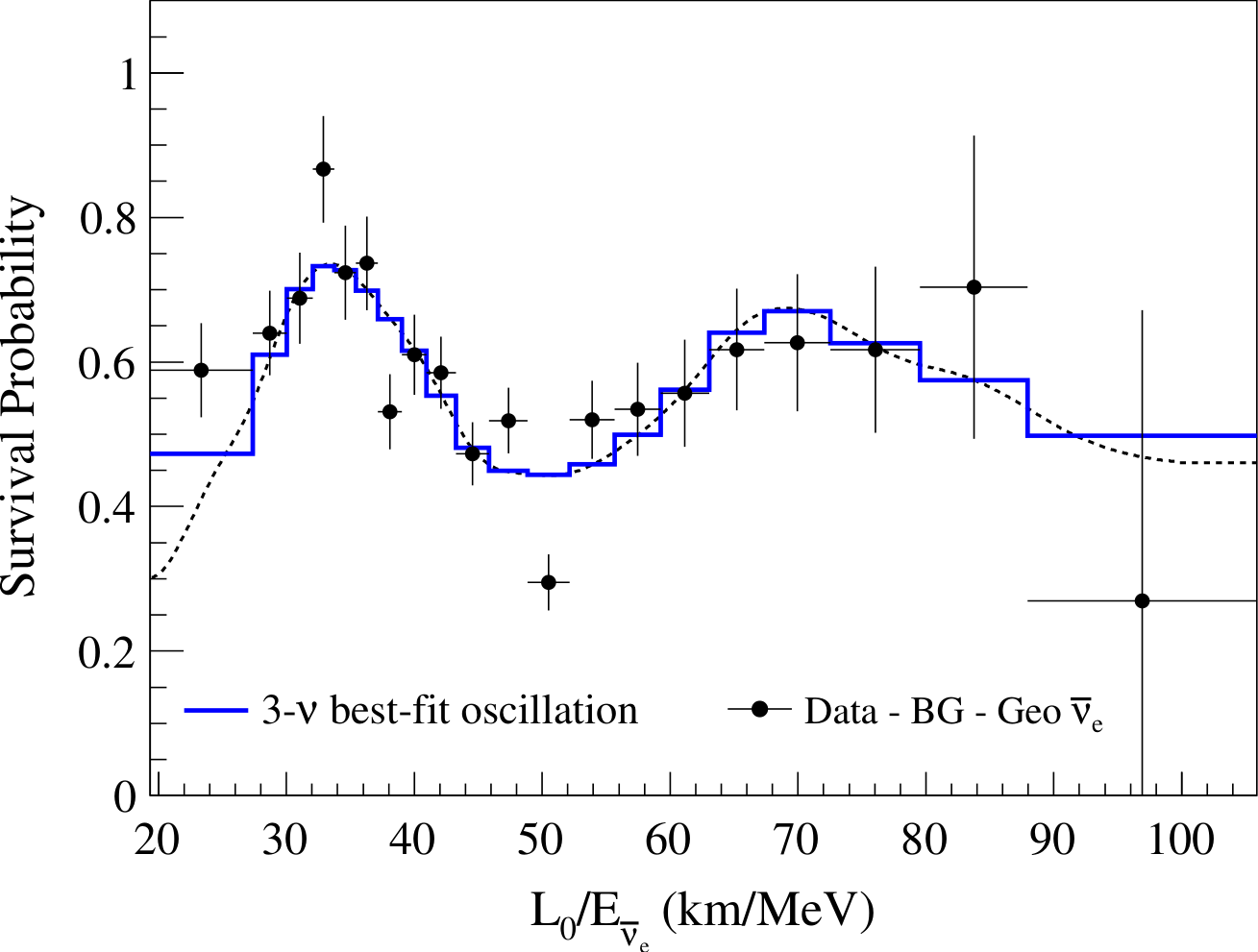
Original figure: KamLAND, Phys. Rev. D 88, 033001 (2013), Fig. 5, doi:10.1103/PhysRevD.88.033001. Not our work; shown for comparison, all rights with the authors and publisher.
Geo-ν̄e event numbers: (a) regions in ((N_U − N_Th)/(N_U + N_Th), N_U + N_Th); (b) Δχ² of N_U + N_Th for chondritic Th/U · Fig. 7
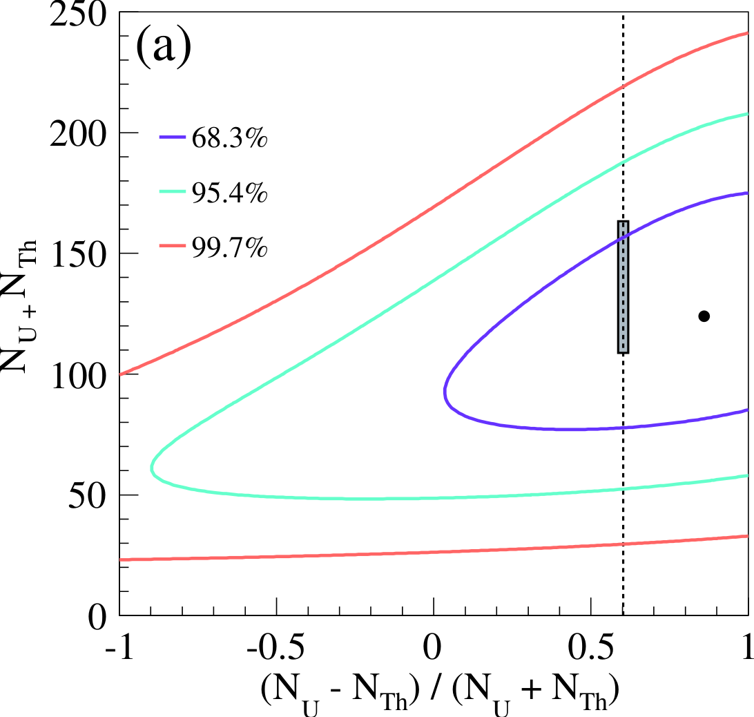
Original figure: KamLAND, Phys. Rev. D 88, 033001 (2013), Fig. 7, doi:10.1103/PhysRevD.88.033001. Not our work; shown for comparison, all rights with the authors and publisher.
Known limitations
- Spectra, backgrounds, efficiencies and geo-ν̄e shapes are extracted from the vector graphics of the paper's Figs. 3 and 6 (17 bins of 0.425 MeV per period); KamLAND fits the unbinned, time-dependent data.
- Reactor operation is known from PRIS only as annual load factors per unit; within a year, operation is placed by the shutdown, suspension and restart dates, and KamLAND's live time is spread uniformly over each period.
- Fission fractions are KamLAND's averages for all reactors; Korean reactors come out at 4.0 % of the no-oscillation events (KamLAND: 4.9 %), other reactors worldwide are fixed at the paper's 1.1 %.
- Geo ν̄e (Fig. 7): the oscillation parameters are fixed at the paper's combined values (tan²θ₁₂ = 0.436, Δm²₂₁ = 7.53×10⁻⁵ eV², sin²θ₁₃ = 0.023) rather than constrained by the solar and accelerator data in the fit; the chondritic Th/U ratio is represented by the reference model's N_Th/N_U = 27/109. Newtrinos prefers about 20 more geo events than KamLAND (0.7σ): the binned, time-integrated spectra per period carry less information to separate geo ν̄e from the low-energy reactor spectrum and ¹³C(α,n) than KamLAND's unbinned, time-dependent fit. Fig. 5: Newtrinos points per prompt-energy bin (data minus Newtrinos backgrounds and geo ν̄e over the Newtrinos no-oscillation expectation, statistical errors); KamLAND's points and histogram (data/extract_fig5_fig7a.py) use their own L₀/E bins.
- The contours use a coarse validation grid and are shown zoomed on the allowed region; the solar and combined regions of the original figure are not reproduced. The official KamLAND-only contours and profiles (data/fig4a_*.csv) are extracted from the vector graphics of the paper's figure (data/extract_fig4a.py).
Reproduce
git clone https://github.com/Newtrinos-org/Newtrinos.jl.git && cd Newtrinos.jl && git checkout c6612c255a- Download reproduce.jl and the
data/folder of this entry into an empty directory. julia -t 8 --project=/path/to/Newtrinos.jl reproduce.jl
# Reproduction of KamLAND, Phys. Rev. D 88, 033001 (2013) [arXiv:1303.4667], KamLAND-only three-flavour analysis with
# Newtrinos.jl (module `kamland`: the three data-taking periods, reactor prediction from the IAEA PRIS power histories
# with the common `reactor_flux` model). θ₁₃ free, as in the paper's KamLAND-only fit.
# Run from this directory with the Newtrinos.jl environment at the pinned commit:
#   julia -t 32 --project=<path to Newtrinos.jl> reproduce.jl
using Newtrinos, Distributions, DataStructures, FileIO, CairoMakie, CSV, DataFrames, Printf
using BAT: distprod

cd(@__DIR__); mkpath("ours"); mkpath("results"); mkpath("cache")
const K = Newtrinos.kamland

experiments = (kamland = K.configure(),)
likelihood = Newtrinos.generate_likelihood(experiments)
p = merge(Newtrinos.get_params(experiments), (θ₁₂ = atan(sqrt(0.48)), θ₁₃ = asin(sqrt(0.02)), Δm²₂₁ = 7.5e-5))
priors = merge(Newtrinos.get_priors(experiments), (Δm²₃₁ = p.Δm²₃₁, θ₂₃ = p.θ₂₃, δCP = p.δCP,
               θ₁₃ = Uniform(0.0, asin(sqrt(0.15))), θ₁₂ = Uniform(atan(sqrt(0.2)), atan(sqrt(1.0))), Δm²₂₁ = Uniform(6.6e-5, 8.6e-5)))

best = Newtrinos.find_mle(likelihood, distprod(; priors...), p)
bf = best[3]
# coarse grids: this entry validates the module, it does not aim at smooth publication-quality contours
th12_dm21 = Newtrinos.profile(likelihood, priors, OrderedDict(:θ₁₂ => 15, :Δm²₂₁ => 17), p, cache_dir = "cache/th12_dm21")
dm21 = Newtrinos.profile(likelihood, priors, OrderedDict(:Δm²₂₁ => 41), p, cache_dir = "cache/dm21")
th12 = Newtrinos.profile(likelihood, priors, OrderedDict(:θ₁₂ => 33), p, cache_dir = "cache/th12")
FileIO.save("results/kamland2013.jld2", Dict("th12_dm21" => th12_dm21, "dm21" => dm21, "th12" => th12, "best_fit" => Dict(pairs(bf))))

Δχ²(r) = 2 .* (maximum(r.values.log_posterior) .- r.values.log_posterior)
"best fit and 1σ range from the Δχ² = 1 crossings (linear interpolation between grid points)"
function onesigma(x, y)
    y = y .- minimum(y); i = argmin(y)
    j = findlast(>(1), y[1:i]); lo = j === nothing ? x[1] : x[j] + (1 - y[j]) * (x[j+1] - x[j]) / (y[j+1] - y[j])
    j = findfirst(>(1), y[i:end]); hi = j === nothing ? x[end] : (j += i - 1; x[j-1] + (1 - y[j-1]) * (x[j] - x[j-1]) / (y[j] - y[j-1]))
    x[i], hi - x[i], x[i] - lo
end
dm = onesigma(dm21.axes.Δm²₂₁ .* 1e5, Δχ²(dm21)); t12 = onesigma(tan.(th12.axes.θ₁₂) .^ 2, Δχ²(th12))
CSV.write("results/dm21_profile.csv", DataFrame(dm2_21 = dm21.axes.Δm²₂₁, dchi2 = Δχ²(dm21)))
CSV.write("results/tan2_theta12_profile.csv", DataFrame(tan2_theta12 = tan.(th12.axes.θ₁₂) .^ 2, dchi2 = Δχ²(th12)))
CSV.write("results/th12_dm21.csv", DataFrame(tan2_theta12 = vec([tan(a)^2 for a in th12_dm21.axes.θ₁₂, b in th12_dm21.axes.Δm²₂₁]),
                                              dm2_21 = vec([b for a in th12_dm21.axes.θ₁₂, b in th12_dm21.axes.Δm²₂₁]), dchi2 = vec(Δχ²(th12_dm21))))
open("results/summary.txt", "w") do io
    @printf io "KamLAND-only, θ13 free (Newtrinos | KamLAND PRD 88, 033001)\n"
    @printf io "dm2_21 [1e-5 eV^2]   %.3f +%.3f -%.3f | 7.54 +0.19 -0.18\n" dm...
    @printf io "tan2_theta12         %.3f +%.3f -%.3f | 0.481 +0.092 -0.080\n" t12...
    @printf io "sin2_theta13 (best)  %.3f | 0.010 +0.033 -0.034\n" sin(bf.θ₁₃)^2
    @printf io "geo nu (best fit, x reference model 109 U / 27 Th): U %.2f, Th %.2f | 116 U, 8 Th events\n" bf.kamland_geo_u bf.kamland_geo_th
    for k in (:kamland_energy_scale, :kamland_flux_scale, :kamland_flux_scale_late, :kamland_alpha_n, :kamland_li9)
        @printf io "pull %-24s %+.2f sigma\n" k bf[k]
    end
end
print(read("results/summary.txt", String))

# Fig. 4(a): KamLAND-only regions (95 %, 99 %, 99.73 % C.L., 2 dof) and Δχ² profiles, Newtrinos (blue) overlaid on
# KamLAND's official KamLAND-only curves (black; data/fig4a_*.csv, from the vector graphics of the paper's figure)
offc = CSV.read("data/fig4a_kamland_only_contours.csv", DataFrame; comment = "#")
offp = CSV.read("data/fig4a_kamland_only_profiles.csv", DataFrame; comment = "#")
styles = Dict(95.0 => :dot, 99.0 => :dash, 99.73 => :solid)
fig = Figure(size = (800, 650))
ax = Axis(fig[2, 1], xlabel = "tan²θ₁₂", ylabel = "Δm²₂₁ (10⁻⁴ eV²)")
x = tan.(th12_dm21.axes.θ₁₂) .^ 2; y = th12_dm21.axes.Δm²₂₁ .* 1e4
for g in groupby(offc, :segment)
    lines!(ax, g.tan2_theta12, g.dm2_21 .* 1e4, color = :black, linestyle = styles[Float64(g.cl[1])], linewidth = 1.5)
end
for (lv, ls) in zip((0.95, 0.99, 0.9973), (:dot, :dash, :solid))
    contour!(ax, x, y, Δχ²(th12_dm21), levels = [quantile(Chisq(2), lv)], color = :dodgerblue, linestyle = ls, linewidth = 2.5)
end
lines!(ax, [NaN], [NaN], color = :black, label = "KamLAND (official)")
lines!(ax, [NaN], [NaN], color = :dodgerblue, linewidth = 2.5, label = "Newtrinos")
scatter!(ax, [tan(bf.θ₁₂)^2], [bf.Δm²₂₁ * 1e4], color = :dodgerblue, label = "Newtrinos best fit")
scatter!(ax, [0.481], [0.754], color = :red, marker = :star5, label = "KamLAND best fit")
axislegend(ax, position = :rt)
xlims!(ax, 0.2, 1.0); ylims!(ax, 0.66, 0.86)
axt = Axis(fig[1, 1], ylabel = "Δχ²")
o = offp[offp.variable .== "tan2_theta12", :]; lines!(axt, o.x, o.dchi2, color = :black, linestyle = :dash, linewidth = 1.5)
lines!(axt, tan.(th12.axes.θ₁₂) .^ 2, Δχ²(th12), color = :dodgerblue, linewidth = 2.5)
hlines!(axt, [1, 4, 9], color = :gray, linewidth = 0.5); xlims!(axt, 0.2, 1.0); ylims!(axt, 0, 12); hidexdecorations!(axt, grid = false)
axr = Axis(fig[2, 2], xlabel = "Δχ²")
o = offp[offp.variable .== "dm2_21", :]; lines!(axr, o.dchi2, o.x .* 1e4, color = :black, linestyle = :dash, linewidth = 1.5)
lines!(axr, Δχ²(dm21), dm21.axes.Δm²₂₁ .* 1e4, color = :dodgerblue, linewidth = 2.5)
vlines!(axr, [1, 4, 9], color = :gray, linewidth = 0.5); ylims!(axr, 0.66, 0.86); xlims!(axr, 0, 20); hideydecorations!(axr, grid = false)
colsize!(fig.layout, 2, Relative(0.25)); rowsize!(fig.layout, 1, Relative(0.25))
Label(fig[0, :], "KamLAND only, θ₁₃ free: Newtrinos (blue) vs KamLAND (black); 95 % dotted, 99 % dashed, 99.73 % C.L. solid", fontsize = 13)
save("ours/fig4a_th12_dm21.png", fig)

# Fig. 3: prompt spectra per period with the best-fit contributions (events / 0.425 MeV / day)
a = experiments.kamland.assets; phys = experiments.kamland.physics
μ = K.get_expected(bf, phys, a)
reac = K.reactor_events(bf, phys, a; ε = K.ESCALE_UNC * bf.kamland_energy_scale)
Ec = 0.5 .* (K.EDGES[1:end-1] .+ K.EDGES[2:end])
fig = Figure(size = (650, 950))
for p in 1:3
    pd = a.periods[p]; d = pd.days
    rate = K.rate_factor(bf, a.ds, p)
    acc = pd.acc; an = acc .+ pd.alpha_n .* (1 + a.ds.alpha_n_unc * bf.kamland_alpha_n)
    geo = an .+ pd.geo_u .* bf.kamland_geo_u .+ pd.geo_th .* bf.kamland_geo_th
    ax = Axis(fig[p, 1], ylabel = "events / 0.425 MeV / day", title = "Period $p ($(Int(d)) live days)",
              xlabel = p == 3 ? "E_p (MeV)" : "")
    edges = K.EDGES
    stairs!(ax, edges, vcat(geo, geo[end]) ./ d, step = :post, color = :blue, linewidth = 1)
    barplot!(ax, Ec, geo ./ d, width = 0.425, gap = 0, color = (:blue, 0.25), label = "best-fit geo ν̄e")
    barplot!(ax, Ec, an ./ d, width = 0.425, gap = 0, color = :lightgreen, label = "¹³C(α,n)¹⁶O")
    barplot!(ax, Ec, acc ./ d, width = 0.425, gap = 0, color = :salmon, label = "accidental")
    stairs!(ax, edges, vcat(reac[p] .* rate, 0) ./ d, step = :post, color = :purple, linestyle = :dash, linewidth = 2, label = "best-fit reactor ν̄e")
    stairs!(ax, edges, vcat(μ[p], μ[p][end]) ./ d, step = :post, color = :dodgerblue, linewidth = 2.5, label = "total")
    n = pd.observed
    errorbars!(ax, Ec, n ./ d, sqrt.(n) ./ d, color = :black); scatter!(ax, Ec, n ./ d, color = :black, label = "KamLAND data")
    xlims!(ax, 0, 8.5); ylims!(ax, 0, 0.18)
    p == 3 && axislegend(ax, position = :rt, labelsize = 11)
end
save("ours/fig3_spectra.png", fig)

# ---------------- Fig. 5: (data − background − geo) / no oscillation vs L₀/E (L₀ = 180 km), all periods ----------------
ε = K.ESCALE_UNC * bf.kamland_energy_scale
reac_bf = K.reactor_events(bf, phys, a; ε)
reac_0 = K.reactor_events(merge(bf, (θ₁₂ = 0.0, θ₁₃ = 0.0)), phys, a; ε)
R1 = sum(reac_bf[p] .* K.rate_factor(bf, a.ds, p) for p in 1:3); R0 = sum(reac_0[p] .* K.rate_factor(bf, a.ds, p) for p in 1:3)
Ntot = sum(a.periods[p].observed for p in 1:3)
bgtot = sum(μ[p] .- reac_bf[p] .* K.rate_factor(bf, a.ds, p) for p in 1:3)
LE = 180 ./ (Ec .+ K.ΔE_NU); LEe = 180 ./ (K.EDGES .+ K.ΔE_NU)
ratio = (Ntot .- bgtot) ./ R0; ratio_err = sqrt.(max.(Ntot, 1)) ./ R0
CSV.write("results/fig5_survival_LE.csv", DataFrame(E_lo = K.EDGES[1:end-1], E_hi = K.EDGES[2:end], LE_km_per_MeV = LE,
                                                    ratio = ratio, ratio_err = ratio_err, expected = R1 ./ R0))
k5 = CSV.read("data/fig5_points.csv", DataFrame; comment = "#"); h5 = CSV.read("data/fig5_histogram.csv", DataFrame; comment = "#")
fig = Figure(size = (800, 500))
ax = Axis(fig[1, 1], xlabel = "L₀/E_ν̄ (km/MeV)", ylabel = "Survival probability", title = "Data − BG − geo ν̄e, ratio to no oscillation (all periods)")
for r in eachrow(h5); lines!(ax, [r.LE_lo, r.LE_hi], [r.P, r.P], color = (:blue, 0.5), linewidth = 1.5); end
rangebars!(ax, k5.LE, k5.P_lo, k5.P_hi, color = :gray50); scatter!(ax, k5.LE, k5.P, color = :gray50, label = "KamLAND (Fig. 5, L₀/E bins)")
for b in 1:17; lines!(ax, [LEe[b+1], LEe[b]], fill((R1 ./ R0)[b], 2), color = :dodgerblue, linewidth = 2.5); end
errorbars!(ax, LE, ratio, ratio_err, color = :red); scatter!(ax, LE, ratio, color = :red, label = "Newtrinos: data per prompt bin")
lines!(ax, [NaN], [NaN], color = :dodgerblue, linewidth = 2.5, label = "Newtrinos: 3ν best fit (KamLAND only)")
lines!(ax, [NaN], [NaN], color = (:blue, 0.5), label = "KamLAND: 3ν best fit")
xlims!(ax, 15, 110); ylims!(ax, 0, 1.15); axislegend(ax, position = :rt, labelsize = 11)
save("ours/fig5_survival_LE.png", fig)

# ---------------- Fig. 7: geo-ν̄e event numbers (U, Th), oscillation parameters at the solar + KamLAND + θ₁₃ values ----------------
# (the paper's geo fit "incorporates all available constraints on the oscillation parameters"; here they are fixed at
# tan²θ₁₂ = 0.436, Δm²₂₁ = 7.53e-5 eV², sin²θ₁₃ = 0.023 from the same paper)
NU_ref = sum(sum(pd.geo_u) for pd in a.periods); NTh_ref = sum(sum(pd.geo_th) for pd in a.periods)     # 109 and 27 events
pg = merge(p, (θ₁₂ = atan(sqrt(0.436)), θ₁₃ = asin(sqrt(0.023)), Δm²₂₁ = 7.53e-5))
priors_geo = merge(priors, (θ₁₂ = pg.θ₁₂, θ₁₃ = pg.θ₁₃, Δm²₂₁ = pg.Δm²₂₁, kamland_geo_u = Uniform(0.0, 2.6), kamland_geo_th = Uniform(0.0, 4.0)))
geo2d = Newtrinos.profile(likelihood, priors_geo, OrderedDict(:kamland_geo_u => 27, :kamland_geo_th => 21), pg, cache_dir = "cache/geo2d")
NU = geo2d.axes.kamland_geo_u .* NU_ref; NTh = geo2d.axes.kamland_geo_th .* NTh_ref; χ²g = Δχ²(geo2d)
CSV.write("results/geo_NU_NTh.csv", DataFrame(N_U = vec([u for u in NU, t in NTh]), N_Th = vec([t for u in NU, t in NTh]), dchi2 = vec(χ²g)))
# Fig. 7(b): total geo events with the chondritic Th/U ratio of the reference model (N_Th / N_U = 27 / 109)
s_grid = collect(range(0.0, 2.0, length = 21))
llh_tot = map(s_grid) do s
    pr = merge(priors_geo, (kamland_geo_u = s, kamland_geo_th = s))
    Newtrinos.find_mle(likelihood, distprod(; pr...), merge(pg, (kamland_geo_u = s, kamland_geo_th = s)))[2]
end
Ntot_geo = s_grid .* (NU_ref + NTh_ref); χ²tot = 2 .* (maximum(llh_tot) .- llh_tot)
gt = onesigma(Ntot_geo, χ²tot)
CSV.write("results/geo_total_profile.csv", DataFrame(N_U_plus_N_Th = Ntot_geo, dchi2 = χ²tot))
open("results/summary.txt", "a") do io
    @printf io "geo nu, oscillation parameters fixed at solar+KamLAND+θ13: N_U + N_Th (Th/U chondritic) = %.0f +%.0f -%.0f | 116 +28 -27 (paper)\n" gt...
    i = argmin(χ²g); @printf io "geo nu, U and Th free: best fit N_U = %.0f, N_Th = %.0f\n" NU[i[1]] NTh[i[2]]
end
c7 = CSV.read("data/fig7a_contours.csv", DataFrame; comment = "#")
fig = Figure(size = (1150, 480))
ax = Axis(fig[1, 1], xlabel = "(N_U − N_Th) / (N_U + N_Th)", ylabel = "N_U + N_Th", title = "(a) geo ν̄e events: 68.3 / 95.4 / 99.7 % C.L. (2 dof)")
asym = [(u - t) / (u + t) for u in NU, t in NTh]; tot = [u + t for u in NU, t in NTh]
colors7 = Dict(68.3 => :purple, 95.4 => :mediumseagreen, 99.7 => :red)
for g in groupby(c7, :segment)
    lines!(ax, g.asymmetry, g.N_total, color = (colors7[Float64(g.cl[1])], 0.6), linewidth = 1.5, linestyle = :dash)
end
# contours of Δχ² on the (N_U, N_Th) grid, drawn in the paper's coordinates
for (cl, c) in colors7
    lv = quantile(Chisq(2), cl / 100)
    cs = Makie.Contours.contours(collect(NU), collect(NTh), χ²g, [lv])
    for l in Makie.Contours.levels(cs), line in Makie.Contours.lines(l)
        v = line.vertices
        lines!(ax, [(q[1] - q[2]) / (q[1] + q[2]) for q in v], [q[1] + q[2] for q in v], color = c, linewidth = 2.5)
    end
end
i = argmin(χ²g); scatter!(ax, [asym[i]], [tot[i]], color = :black)
vlines!(ax, [(109 - 27) / 136], color = :black, linestyle = :dot)
lines!(ax, [NaN], [NaN], color = :black, linewidth = 2.5, label = "Newtrinos"); lines!(ax, [NaN], [NaN], color = (:black, 0.6), linestyle = :dash, label = "KamLAND (Fig. 7a)")
axislegend(ax, position = :lt); xlims!(ax, -1, 1); ylims!(ax, 0, 250)
ax2 = Axis(fig[1, 2], xlabel = "N_U + N_Th (Th/U chondritic)", ylabel = "Δχ²", title = "(b) total geo ν̄e events")
lines!(ax2, Ntot_geo, χ²tot, color = :dodgerblue, linewidth = 2.5, label = "Newtrinos")
vspan!(ax2, [116 - 27], [116 + 28], color = (:gray, 0.3), label = "KamLAND: 116 +28 −27")
vlines!(ax2, [136], color = :black, linestyle = :dot, label = "reference model (109 U + 27 Th)")
xlims!(ax2, 0, 280); ylims!(ax2, 0, 25); axislegend(ax2, position = :rt)
save("ours/fig7_geo.png", fig)
print(read("results/summary.txt", String))
Provenance
| Newtrinos.jl commit | c6612c255a (kamland, reactor_flux, osc) |
|---|---|
| Run date | 2026-10-21T16:09:57Z |
| Wall time | 27.6 min (128 threads) |
| Julia | 1.12.5 |
| Machine | AMD EPYC 7702P 64-Core Processor, 128 hardware threads, Linux |
| Environment | newtrinos_Manifest.toml · run.toml |
Downloads
CSV files hold one row per scan point: the scanned and profiled parameters
(sin2_theta23, dm2_32 in eV², dcp in rad, nuisance parameters), dchi2 = −2Δ log L
and the log-likelihood. JLD2 files contain the full NewtrinosResult objects.
| File | Size | SHA-256 |
|---|---|---|
| ours/fig3_spectra.png | 154.6 kB | 1588c7f63c65… |
| ours/fig4a_th12_dm21.png | 239.5 kB | ce6aa2cdaf76… |
| ours/fig5_survival_LE.png | 94.1 kB | c7cd20ed0dc5… |
| ours/fig7_geo.png | 208.3 kB | 0a163a463af1… |
| results/dm21_profile.csv | 1.2 kB | 55fddd5637b2… |
| results/fig5_survival_LE.csv | 1.5 kB | fcc2ee4d8733… |
| results/geo_NU_NTh.csv | 29.8 kB | 78ea8992278d… |
| results/geo_total_profile.csv | 775 B | 4578e98409cc… |
| results/kamland2013.jld2 | 87.8 kB | ffb5f3342c31… |
| results/summary.txt | 709 B | 145b0efd248c… |
| results/tan2_theta12_profile.csv | 1.2 kB | ce96365956d5… |
| results/th12_dm21.csv | 12.5 kB | f92d26b1df59… |