
T2K · Phys. Rev. D 90, 052010 (2014)
Measurement of the inclusive νμ charged current cross section on iron and hydrocarbon in the T2K on-axis neutrino beam
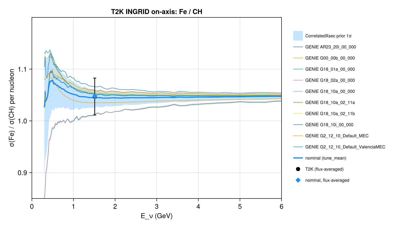
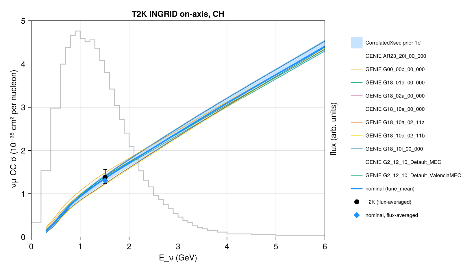
The flux-averaged νμ charged-current inclusive cross sections per nucleon on iron (INGRID modules) and hydrocarbon (Proton Module) at ⟨Eν⟩ = 1.51 GeV, full phase space, and their ratio, compared with the cross sections carried by Newtrinos.jl (module xsec): the ten GENIE tunes of generator_sigma (⁵⁶Fe and CH per nucleon) and the nominal model of CorrelatedXsec (the mean of the tunes) with its prior 1σ band, averaged with the official T2K νμ flux at the Proton Module. The target dependence is reproduced: σ(Fe)/σ(CH) = 1.048 ± 0.017 (prior) for the nominal against 1.047 ± 0.036 measured (tunes 1.015–1.067; the paper's NEUT 1.037, GENIE 1.044). The nominal absolute cross sections, 1.36 ± 0.08 (Fe) and 1.30 ± 0.08 (CH) × 10⁻³⁸ cm², are 6 % below the data, 1.44 +0.19/−0.16 and 1.38 +0.18/−0.15, well within the measurement's uncertainty; the tunes span 1.26–1.50 (Fe) and 1.19–1.42 (CH), the paper's NEUT and GENIE give 1.40/1.35 and 1.24/1.19.
Figures
σ(Fe)/σ(CH) per nucleon: T2K vs the GENIE tunes and the CorrelatedXsec nominal with its prior 1σ band · Fig. 17
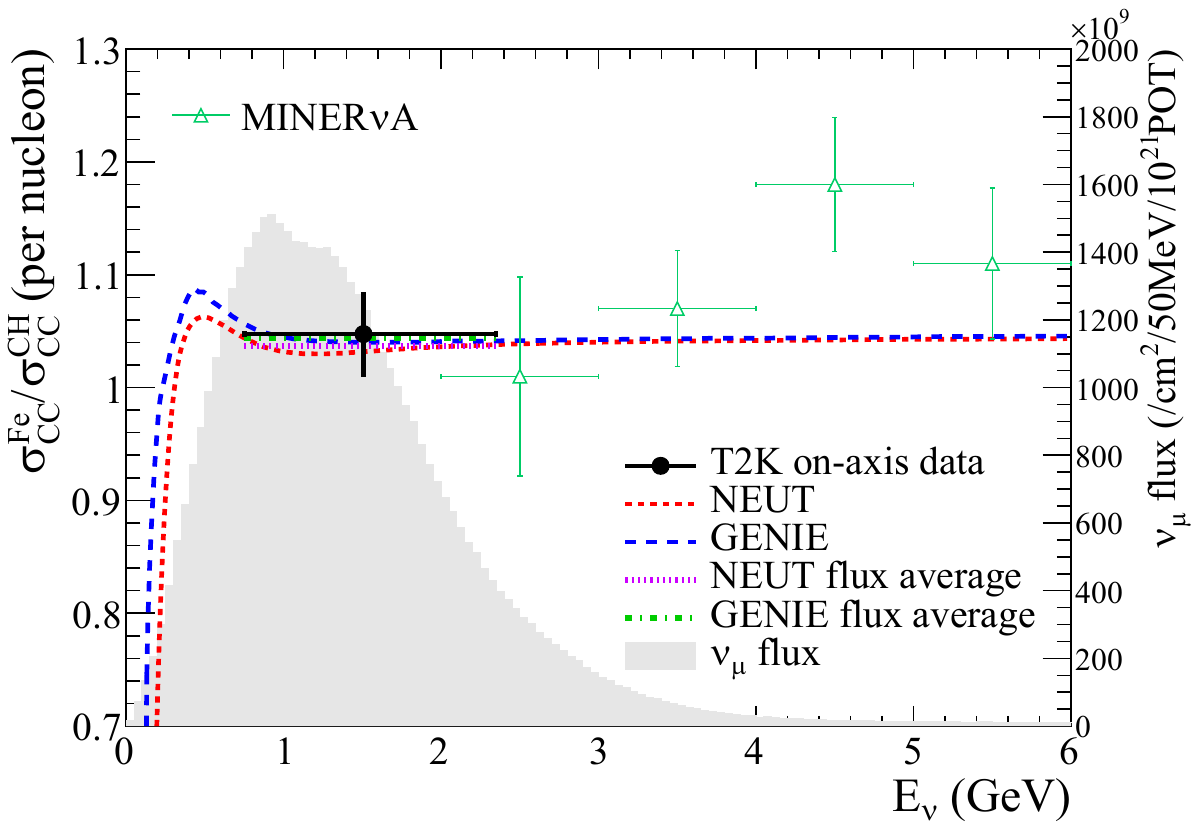
Original figure: T2K, Phys. Rev. D 90, 052010 (2014), Fig. 17, doi:10.1103/PhysRevD.90.052010. Not our work; shown for comparison, all rights with the authors and publisher.
νμ CC σ per nucleon on iron and the flux-averaged values · Fig. 16 (Fe)
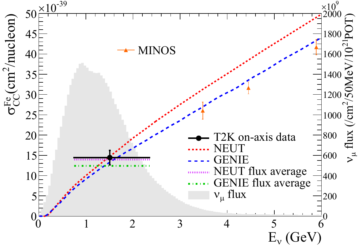
Original figure: T2K, Phys. Rev. D 90, 052010 (2014), Fig. 16 (Fe), doi:10.1103/PhysRevD.90.052010. Not our work; shown for comparison, all rights with the authors and publisher.
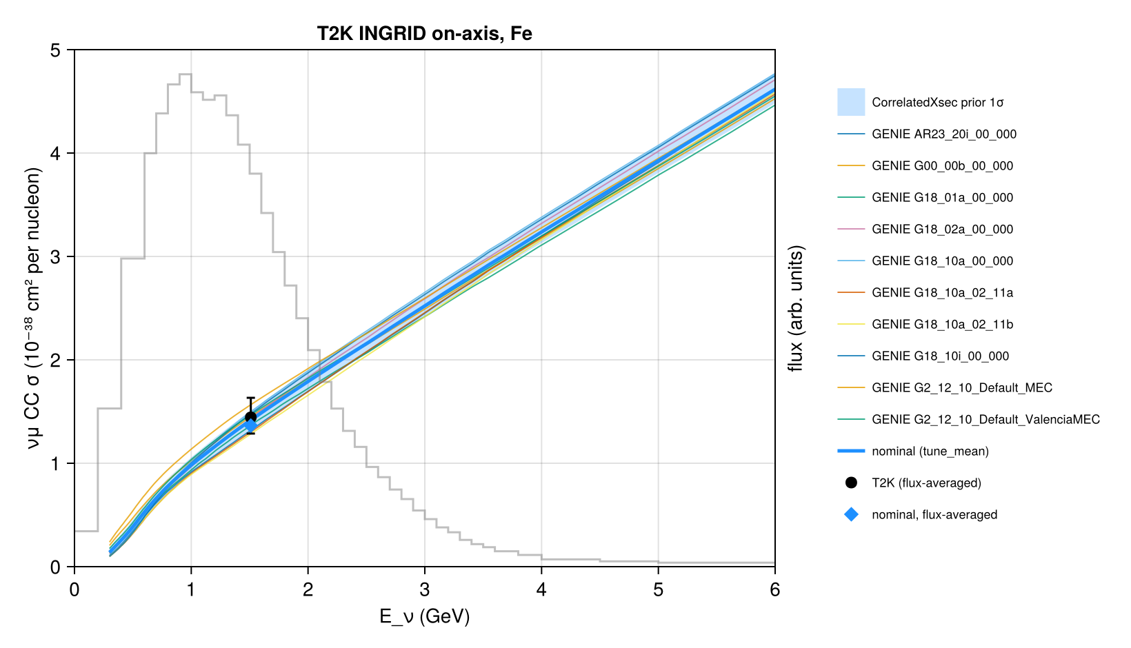
νμ CC σ per nucleon on CH and the flux-averaged values · Fig. 16 (CH)
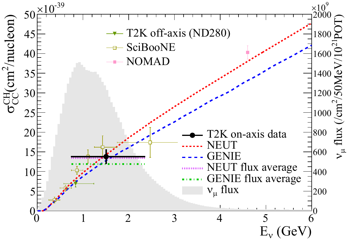
Original figure: T2K, Phys. Rev. D 90, 052010 (2014), Fig. 16 (CH), doi:10.1103/PhysRevD.90.052010. Not our work; shown for comparison, all rights with the authors and publisher.
Known limitations
- Flux: the official release (ingriddata-numu-ccqe-xs-2015) provides the Proton Module flux, which its README states was used for this measurement. The iron modules' flux is not public; according to the paper its normalisation differs by about 1 % (Φ_Fe/Φ_CH = 0.991) and the digitised flux of the paper agrees in shape to 1–2 %, so the Proton Module flux is used for both. The released flux gives ⟨E⟩ = 1.537 GeV (paper 1.51 GeV).
- Per nucleon without isoscalar correction (iron: 26 protons, 30 neutrons; CH: 7 protons, 6 neutrons per 13 nucleons), as the paper.
- The measurement is extrapolated to full phase space with NEUT; its 12 % systematic uncertainty is dominated by the flux.
- The paper does not state the NEUT and GENIE versions of its predictions.
Reproduce
git clone https://github.com/Newtrinos-org/Newtrinos.jl.git && cd Newtrinos.jl && git checkout 78e71c310b- Download reproduce.jl and the
data/folder of this entry into an empty directory. julia -t 8 --project=/path/to/Newtrinos.jl reproduce.jl
# T2K INGRID on-axis νμ CC inclusive cross sections per nucleon on iron and hydrocarbon (CH) and their ratio, flux
# averaged at ⟨E⟩ = 1.51 GeV, full phase space (PRD 90, 052010 (2014), in data/), compared with the cross sections of
# Newtrinos.jl (module `xsec`): the GENIE tunes (`generator_sigma`, ⁵⁶Fe and CH per nucleon) and the reference model of
# `CorrelatedXsec` with its prior 1σ band (Fe and CH sampled jointly). The models are averaged with the official T2K
# νμ flux at the INGRID Proton Module (data release ingriddata-numu-ccqe-xs-2015, which the release states was used for
# this measurement; data/flux_ProtonModule.csv); the iron modules see the same flux shape to 1–2 %.
# Run from this directory with the Newtrinos.jl environment at the pinned commit:
#   julia --project=<path to Newtrinos.jl> reproduce.jl
using Newtrinos, CairoMakie, CSV, DataFrames, Printf, Statistics, Random, Distributions

cd(@__DIR__); mkpath("ours"); mkpath("results")
const X = Newtrinos.xsec

readc(f) = CSV.read(f, DataFrame; comment = "#", normalizenames = true)
A = readc("data/flux_averaged.csv")
Rt = readc("data/ratio.csv")
F = readc("data/flux_ProtonModule.csv")
dFe, dCH = A[A.target .== "Fe", :][1, :], A[A.target .== "CH", :][1, :]

# fine grid with the flux histogram (constant within its bins)
Ef = collect(range(0.01, F.E_hi[end], length = 6000))
Φ = [F.flux_per100MeV[clamp(searchsortedlast(F.E_lo, e), 1, nrow(F))] for e in Ef]
fluxavg(σ) = sum(Φ .* σ) / sum(Φ)
@printf("⟨E⟩ of the flux: %.3f GeV (paper 1.51)\n", fluxavg(Ef))

tab = X.load_table()
at(v, e) = X.at_energies(tab.E, v, e)
TUNES = Symbol.(sort(tab.tunes))
σ_tune(t, target, e) = at(sum(X.generator_sigma(t, target, :numu, false, :CC)), e) .* e

xs = X.configure(X.CorrelatedXsec())
ref = xs.cfg.reference
sf = Dict(tg => xs.sigma(Ef; flavour = :numu, anti = false, current = :CC, target = tg) for tg in (:Fe, :CH))
avg(p, tg) = fluxavg(sf[tg](p) .* Ef)
rng = MersenneTwister(1)
draw() = map(p -> p isa Distribution ? rand(rng, p) : p, xs.priors)
samples = [draw() for _ in 1:500]
p0 = xs.params
sFe = [avg(p, :Fe) for p in samples]; sCH = [avg(p, :CH) for p in samples]; sR = sFe ./ sCH

rows = [(model = "$(ref) (nominal)", Fe = avg(p0, :Fe), CH = avg(p0, :CH), Fe_over_CH = avg(p0, :Fe) / avg(p0, :CH))]
push!(rows, (model = "prior 1σ of the nominal", Fe = std(sFe), CH = std(sCH), Fe_over_CH = std(sR)))
for t in TUNES
    a, b = fluxavg(σ_tune(t, :Fe, Ef)), fluxavg(σ_tune(t, :CH, Ef))
    push!(rows, (model = string(t), Fe = a, CH = b, Fe_over_CH = a / b))
end
push!(rows, (model = "paper: NEUT", Fe = dFe.NEUT_pred, CH = dCH.NEUT_pred, Fe_over_CH = Rt.NEUT_pred[1]))
push!(rows, (model = "paper: GENIE", Fe = dFe.GENIE_pred, CH = dCH.GENIE_pred, Fe_over_CH = Rt.GENIE_pred[1]))
push!(rows, (model = "T2K data", Fe = dFe.sigma_1e_38cm2_per_nucleon, CH = dCH.sigma_1e_38cm2_per_nucleon, Fe_over_CH = Rt.value[1]))
out = DataFrame(rows)
out.Fe = round.(out.Fe, digits = 4); out.CH = round.(out.CH, digits = 4); out.Fe_over_CH = round.(out.Fe_over_CH, digits = 4)
CSV.write("results/flux_averaged.csv", out)
show(stdout, out, allrows = true); println()

# figures: σ(E) per nucleon for Fe and CH with the flux-averaged values, and the ratio Fe/CH
E = collect(range(0.3, 6.0, length = 300))
sig = Dict(tg => xs.sigma(E; flavour = :numu, anti = false, current = :CC, target = tg) for tg in (:Fe, :CH))
q(M, a) = [quantile(r, a) for r in eachrow(M)]
for (tg, d, name) in ((:Fe, dFe, "xsec_Fe"), (:CH, dCH, "xsec_CH"))
    M = reduce(hcat, [sig[tg](p) .* E for p in samples])
    fig = Figure(size = (820, 470))
    ax = Axis(fig[1, 1], xlabel = "E_ν (GeV)", ylabel = "νμ CC σ (10⁻³⁸ cm² per nucleon)", title = "T2K INGRID on-axis, $(tg)",
              limits = (0, 6, 0, 5))
    axf = Axis(fig[1, 1], yaxisposition = :right, ylabel = "flux (arb. units)", limits = (0, 6, 0, nothing))
    hidexdecorations!(axf); hideydecorations!(axf, label = false)
    stairs!(axf, vcat(F.E_lo, F.E_hi[end]), vcat(F.flux_per100MeV, F.flux_per100MeV[end]), step = :post, color = (:gray, 0.5))
    band!(ax, E, q(M, 0.16), q(M, 0.84), color = (:dodgerblue, 0.25), label = "CorrelatedXsec prior 1σ")
    for (i, t) in enumerate(TUNES)
        lines!(ax, E, σ_tune(t, tg, E), color = (Makie.wong_colors()[mod1(i, 7)], 0.8), linewidth = 1, label = "GENIE $(t)")
    end
    lines!(ax, E, sig[tg](p0) .* E, color = :dodgerblue, linewidth = 2.5, label = "nominal ($(ref))")
    errorbars!(ax, [dCH.mean_E], [d.sigma_1e_38cm2_per_nucleon], [d.syst_down], [d.syst_up], color = :black, whiskerwidth = 6)
    scatter!(ax, [dCH.mean_E], [d.sigma_1e_38cm2_per_nucleon], color = :black, markersize = 12, label = "T2K (flux-averaged)")
    scatter!(ax, [dCH.mean_E], [avg(p0, tg)], color = :dodgerblue, marker = :diamond, markersize = 12, label = "nominal, flux-averaged")
    Legend(fig[1, 2], ax, framevisible = false, labelsize = 9)
    save("ours/$(name).png", fig)
end
MR = reduce(hcat, [sig[:Fe](p) ./ sig[:CH](p) for p in samples])
fig = Figure(size = (820, 470))
ax = Axis(fig[1, 1], xlabel = "E_ν (GeV)", ylabel = "σ(Fe) / σ(CH) per nucleon", title = "T2K INGRID on-axis: Fe / CH", limits = (0, 6, 0.85, 1.2))
band!(ax, E, q(MR, 0.16), q(MR, 0.84), color = (:dodgerblue, 0.25), label = "CorrelatedXsec prior 1σ")
for (i, t) in enumerate(TUNES)
    lines!(ax, E, σ_tune(t, :Fe, E) ./ σ_tune(t, :CH, E), color = (Makie.wong_colors()[mod1(i, 7)], 0.8), linewidth = 1, label = "GENIE $(t)")
end
lines!(ax, E, sig[:Fe](p0) ./ sig[:CH](p0), color = :dodgerblue, linewidth = 2.5, label = "nominal ($(ref))")
e = sqrt(Rt.stat[1]^2 + Rt.syst[1]^2)
errorbars!(ax, [Rt.mean_E[1]], [Rt.value[1]], [e], color = :black, whiskerwidth = 6)
scatter!(ax, [Rt.mean_E[1]], [Rt.value[1]], color = :black, markersize = 12, label = "T2K (flux-averaged)")
scatter!(ax, [Rt.mean_E[1]], [avg(p0, :Fe) / avg(p0, :CH)], color = :dodgerblue, marker = :diamond, markersize = 12, label = "nominal, flux-averaged")
Legend(fig[1, 2], ax, framevisible = false, labelsize = 9)
save("ours/ratio.png", fig)
Provenance
| Newtrinos.jl commit | 78e71c310b (xsec (generator_sigma, CorrelatedXsec)) |
|---|---|
| Run date | 2026-10-12T12:23:11Z |
| Wall time | 1.4 min (4 threads) |
| Julia | 1.12.5 |
| Machine | AMD EPYC 7702P 64-Core Processor, 128 hardware threads, Linux |
| Environment | newtrinos_Manifest.toml · run.toml |
Downloads
CSV files hold one row per scan point: the scanned and profiled parameters
(sin2_theta23, dm2_32 in eV², dcp in rad, nuisance parameters), dchi2 = −2Δ log L
and the log-likelihood. JLD2 files contain the full NewtrinosResult objects.
| File | Size | SHA-256 |
|---|---|---|
| ours/ratio.png | 177.7 kB | de12bb257ab0… |
| ours/xsec_CH.png | 194.5 kB | e91294432be6… |
| ours/xsec_Fe.png | 211.5 kB | 4b1db057dcb5… |
| results/flux_averaged.csv | 573 B | dc079ca51a58… |