
IceCube Collaboration · Phys. Rev. Lett. 120, 071801 (2018)
Measurement of Atmospheric Neutrino Oscillations at 6–56 GeV with IceCube DeepCore
Atmospheric νμ disappearance with three years of IceCube DeepCore data (2012–2015, 6–56 GeV), reproduced with the Newtrinos module deepcore_3y, built on the public three-year high-statistics sample ("sample B"), which the release describes as a very close variant of the sample of this paper. Oscillation inputs as in the paper (Δm²₂₁ = 7.53·10⁻⁵ eV², sin²θ₁₂ = 0.304, sin²θ₁₃ = 0.0217, δCP = 0, standard ντ); profile likelihood on a 17 × 17 grid in (sin²θ₂₃, Δm²₃₂) for each ordering, compared point by point with the official Δχ² maps and the Feldman–Cousins contour of the paper's data release, plus data/MC comparisons at the best fit.
Figures
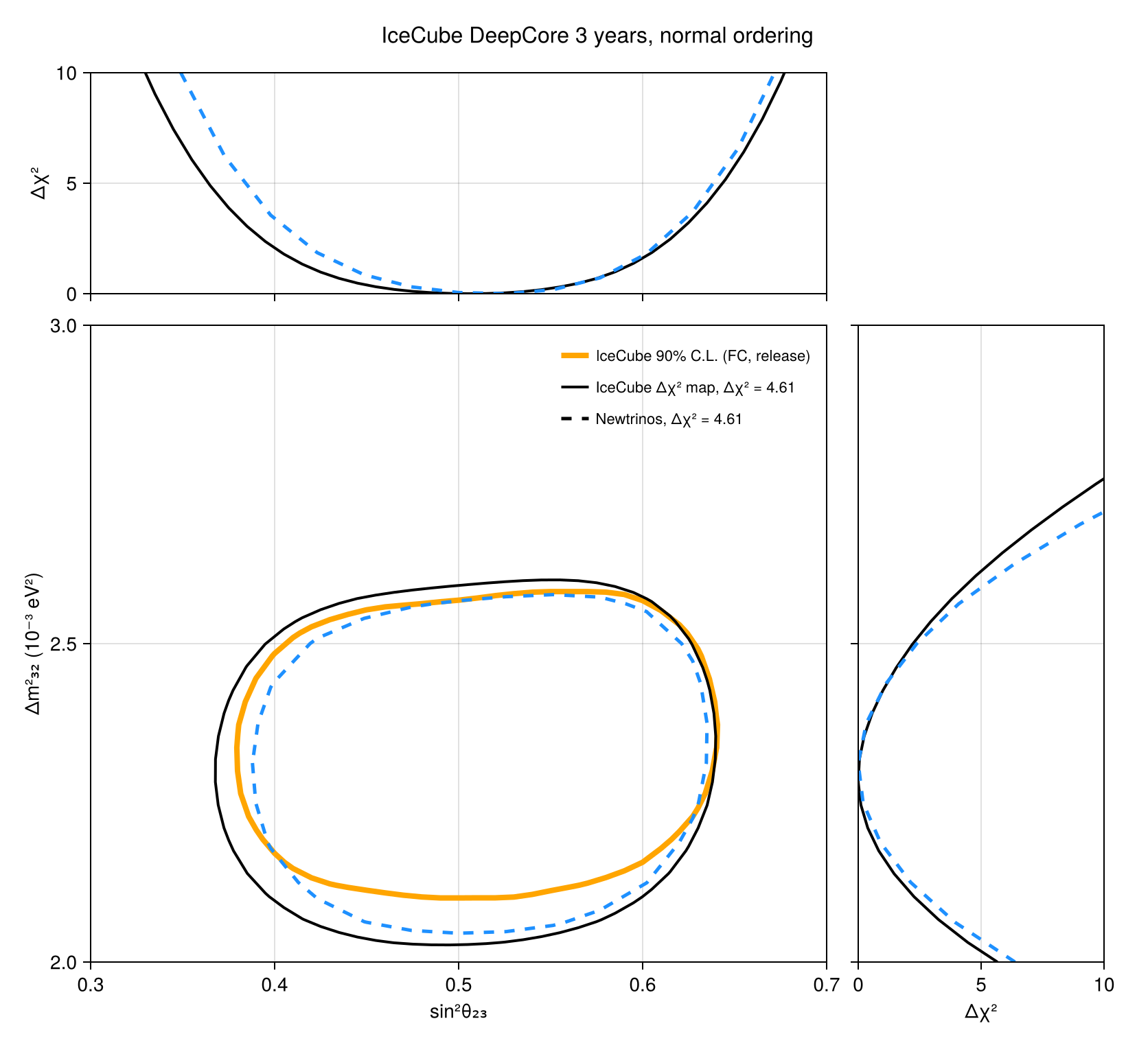
90% C.L. region in (sin²θ₂₃, Δm²₃₂) and 1D profiles, normal ordering · Fig. 3
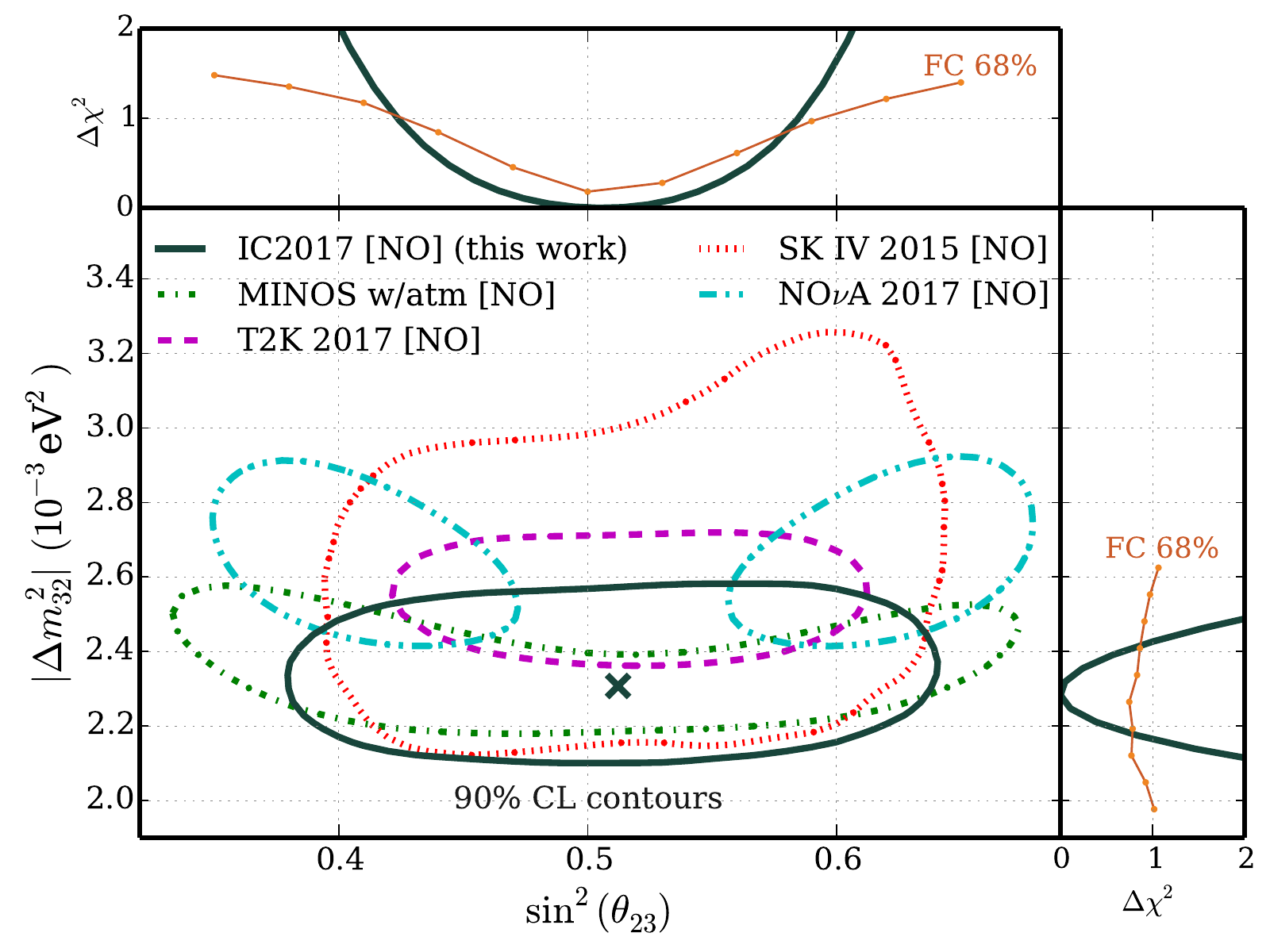
Original figure: IceCube Collaboration, Phys. Rev. Lett. 120, 071801 (2018), Fig. 3, doi:10.1103/PhysRevLett.120.071801. Not our work; shown for comparison, all rights with the authors and publisher.
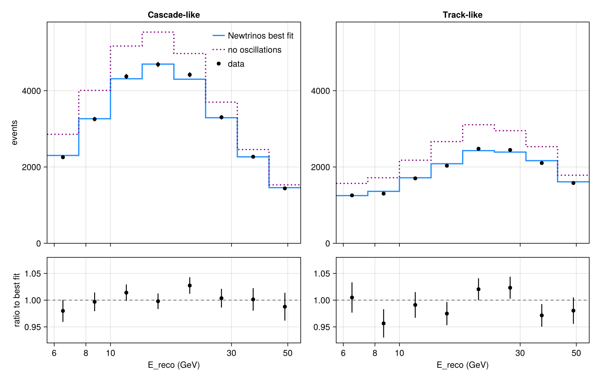
Data and best-fit expectation projected onto reconstructed energy · Fig. 1
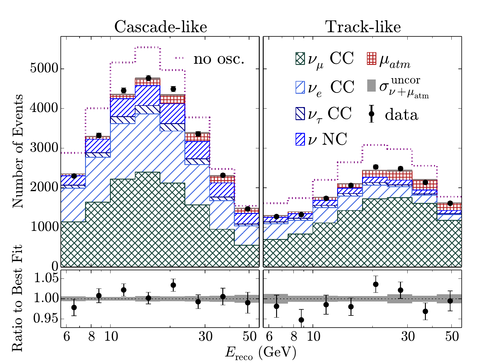
Original figure: IceCube Collaboration, Phys. Rev. Lett. 120, 071801 (2018), Fig. 1, doi:10.1103/PhysRevLett.120.071801. Not our work; shown for comparison, all rights with the authors and publisher.
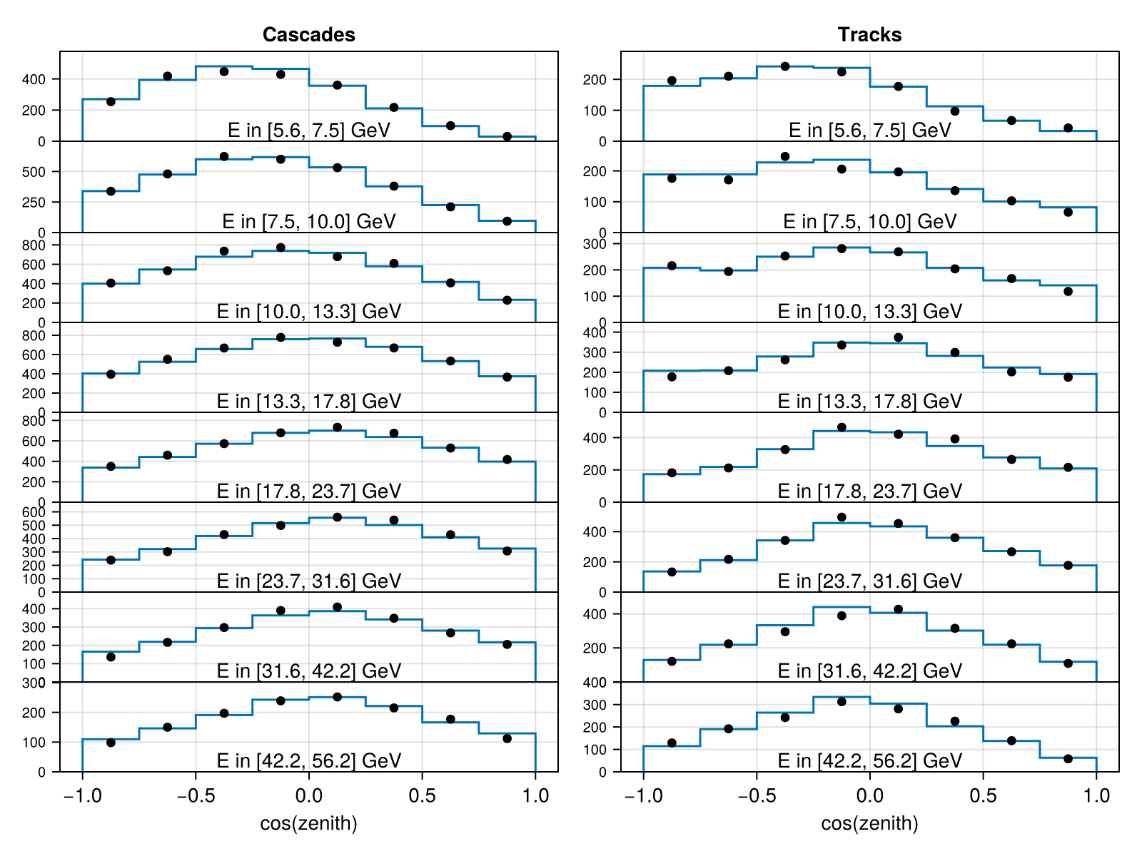
Data and best-fit expectation in all analysis bins · Supplemental Material, best-fit per-bin figure
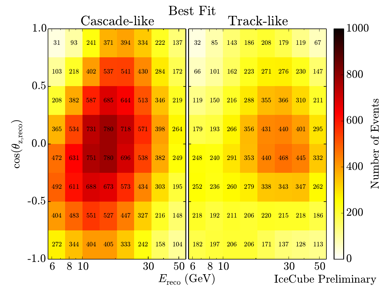
Original figure: IceCube Collaboration, Phys. Rev. Lett. 120, 071801 (2018), Supplemental Material, best-fit per-bin figure, doi:10.1103/PhysRevLett.120.071801. Not our work; shown for comparison, all rights with the authors and publisher.
Known limitations
- Best fit (NO): Δm²₃₂ = 2.312·10⁻³ eV² (paper 2.31), sin²θ₂₃ = 0.526 (paper 0.51; flat profile around maximal mixing). The profiled Δχ² differs from the official maps by a median of 0.8 (NO) and 1.0 (IO), at most 4.5, in the region with Δχ² < 12. Our Δχ² = 4.61 contour is somewhat smaller than the one from the official Δχ² map, mainly in the lower octant and at low Δm²₃₂, and lies close to the official Feldman–Cousins contour.
- Sample and systematics: the public sample is a close variant of the paper's. The module's nuisances differ from the paper's Table I: five Barr flux parameters instead of the paper's two hadronic-flux parameters, the Barr νe/νμ ratio instead of a 20 % νe normalisation, no M_A(RES) parameter, and ice absorption and scattering hyperplanes as prescribed by the release for sample B.
- Data/MC: the observed counts are identical to the paper's; the data/best-fit ratios in reconstructed energy follow the paper's pattern within about 1–2 %.
- The ντ-appearance result of the same sample (Phys. Rev. D 99, 032007) is not covered here; the module scales only ντ CC events (nutau_cc_norm), so only that paper's CC-only result is reproducible.
Reproduce
git clone https://github.com/Newtrinos-org/Newtrinos.jl.git && cd Newtrinos.jl && git checkout e1b5a89439- Download reproduce.jl and the
data/folder of this entry into an empty directory. julia -t 8 --project=/path/to/Newtrinos.jl reproduce.jl
# IceCube DeepCore 3-year oscillation measurement, IceCube Collaboration, Phys. Rev. Lett. 120, 071801 (2018),
# reproduced with Newtrinos.jl (module `deepcore_3y`, built on the public 3-year high-statistics sample, "sample B",
# doi:10.21234/ac23-ra43, which the release describes as a very close variant of the sample of this paper).
# Compared with the official Δχ² maps and Feldman-Cousins contour of the paper's data release (doi:10.21234/B4105H).
# Run from this directory with the Newtrinos.jl environment at the pinned commit:
#   julia -t 16 --project=<path to Newtrinos.jl> reproduce.jl
using Newtrinos, Statistics, Distributions, DataStructures, FileIO, CairoMakie, CSV, DataFrames, Printf, DelimitedFiles

cd(@__DIR__); mkpath("ours"); mkpath("results"); mkpath("cache")
const N = 17

experiments = (deepcore_3y = Newtrinos.deepcore_3y.configure(),)
lik = Newtrinos.generate_likelihood(experiments)
p0 = Newtrinos.get_params(experiments)
# oscillation inputs fixed as in the paper: Δm²₂₁ = 7.53e-5 eV², sin²θ₁₂ = 0.304, sin²θ₁₃ = 0.0217, δCP = 0; ντ standard
fixed = (Δm²₂₁ = 7.53e-5, θ₁₂ = asin(sqrt(0.304)), θ₁₃ = asin(sqrt(0.0217)), δCP = 0.0, nutau_cc_norm = 1.0)
p0 = merge(p0, fixed)
base = merge(Newtrinos.get_priors(experiments), fixed)

# grid: sin²θ₂₃ 0.30–0.70 (uniform in θ₂₃), |Δm²₃₂| 2.0–3.0e-3 eV²; Δm²₃₁ = Δm²₃₂ + Δm²₂₁
scan(ord) = merge(base, (θ₂₃ = Uniform(asin(sqrt(0.30)), asin(sqrt(0.70))),
                         Δm²₃₁ = ord == :NO ? Uniform(2.0e-3 + fixed.Δm²₂₁, 3.0e-3 + fixed.Δm²₂₁) :
                                              Uniform(-3.0e-3 + fixed.Δm²₂₁, -2.0e-3 + fixed.Δm²₂₁)))
start(ord) = merge(p0, (θ₂₃ = asin(sqrt(0.5)), Δm²₃₁ = (ord == :NO ? 1 : -1) * 2.5e-3 + fixed.Δm²₂₁))
res = OrderedDict(ord => Newtrinos.profile(lik, scan(ord), OrderedDict(:θ₂₃ => N, :Δm²₃₁ => N), start(ord),
                                           cache_dir = "cache/$ord") for ord in (:NO, :IO))
FileIO.save("results/deepcore_3y_profile.jld2", Dict(String(k) => v for (k, v) in res))

# Δχ² within each ordering (relative to that ordering's minimum, as in the release maps)
Δχ²(r) = 2 .* (maximum(r.values.log_posterior) .- r.values.log_posterior)
ss(r) = sin.(r.axes.θ₂₃) .^ 2
dm32(r) = r.axes.Δm²₃₁ .- fixed.Δm²₂₁

# official maps (regular 51 × 51 grids), bilinear interpolation at our grid points
function official(file)
    d = readdlm(file, skipstart = 1)
    dm = sort(unique(d[:, 1])); s2 = sort(unique(d[:, 2]))
    M = fill(NaN, length(dm), length(s2))
    for r in eachrow(d); M[searchsortedfirst(dm, r[1]), searchsortedfirst(s2, r[2])] = r[3]; end
    function at(x, y)                          # x = sin²θ₂₃, y = Δm²₃₂
        i = clamp(searchsortedlast(dm, y), 1, length(dm) - 1); j = clamp(searchsortedlast(s2, x), 1, length(s2) - 1)
        ty = (y - dm[i]) / (dm[i+1] - dm[i]); tx = (x - s2[j]) / (s2[j+1] - s2[j])
        (1 - ty) * (1 - tx) * M[i, j] + ty * (1 - tx) * M[i+1, j] + (1 - ty) * tx * M[i, j+1] + ty * tx * M[i+1, j+1]
    end
    (dm = dm, s2 = s2, M = M, at = at)
end
OFF = Dict(:NO => official("data/chi2_map_NH.dat"), :IO => official("data/chi2_map_IH.dat"))
fc = readdlm("data/IC2017_90CL_FC.dat", skipstart = 1)

rows = []
for (ord, r) in res, (i, x) in enumerate(ss(r)), (j, y) in enumerate(dm32(r))
    push!(rows, (ordering = String(ord), sin2_theta23 = x, dm2_32 = y, dchi2_newtrinos = Δχ²(r)[i, j],
                 dchi2_official = OFF[ord].at(x, y)))
end
tab = DataFrame(rows)
CSV.write("results/dchi2_vs_official.csv", tab)

# ---- figure: 90% C.L. (NO), Wilks Δχ² = 4.61 and the official FC contour, with 1D profiles
fig = Figure(size = (820, 760))
r = res[:NO]; o = OFF[:NO]
ax = Axis(fig[2, 1], xlabel = "sin²θ₂₃", ylabel = "Δm²₃₂ (10⁻³ eV²)", limits = (0.3, 0.7, 2.0, 3.0))
lines!(ax, fc[:, 1], fc[:, 2], color = :orange, linewidth = 4, label = "IceCube 90% C.L. (FC, release)")
contour!(ax, o.s2, o.dm .* 1e3, permutedims(o.M), levels = [4.61], color = :black, linewidth = 2, label = "IceCube Δχ² map, Δχ² = 4.61")
contour!(ax, ss(r), dm32(r) .* 1e3, Δχ²(r), levels = [4.61], color = :dodgerblue, linewidth = 2.5, linestyle = :dash,
         label = "Newtrinos, Δχ² = 4.61")
axislegend(ax, position = :rt, framevisible = false, labelsize = 11)
axt = Axis(fig[1, 1], ylabel = "Δχ²", limits = (0.3, 0.7, 0, 10), xticklabelsvisible = false)
lines!(axt, o.s2, vec(minimum(o.M, dims = 1)), color = :black, linewidth = 2)
lines!(axt, ss(r), vec(minimum(Δχ²(r), dims = 2)), color = :dodgerblue, linewidth = 2.5, linestyle = :dash)
axr = Axis(fig[2, 2], xlabel = "Δχ²", limits = (0, 10, 2.0, 3.0), yticklabelsvisible = false)
lines!(axr, vec(minimum(o.M, dims = 2)), o.dm .* 1e3, color = :black, linewidth = 2)
lines!(axr, vec(minimum(Δχ²(r), dims = 1)), dm32(r) .* 1e3, color = :dodgerblue, linewidth = 2.5, linestyle = :dash)
rowsize!(fig.layout, 1, Relative(0.25)); colsize!(fig.layout, 2, Relative(0.25))
Label(fig[0, 1:2], "IceCube DeepCore 3 years, normal ordering", fontsize = 16)
save("ours/fig3_contours.png", fig)

# ---- data/MC at the best fit (NO)
bf = Newtrinos.bestfit(res[:NO])
X = experiments.deepcore_3y
# (a) all analysis bins: the module's plot of the observed and expected counts (cf. the paper's supplemental figure)
save("ours/datamc_bestfit.png", X.plot(bf))
# (b) projection onto reconstructed energy, as in the paper's Fig. 1, with the no-oscillation expectation
pexp = mean(X.forward_model(bf))                                   # [E, cos θ_z, PID]
pnoosc = mean(X.forward_model(merge(bf, (θ₁₂ = 0.0, θ₁₃ = 0.0, θ₂₃ = 0.0))))
obs = X.assets.observed
edges = X.assets.binning.reco_energy_bin_edges
ec = sqrt.(edges[1:end-1] .* edges[2:end])
fig = Figure(size = (980, 620))
for (k, (pid, name)) in enumerate(((1, "Cascade-like"), (2, "Track-like")))
    ex, no, d = vec(sum(pexp[:, :, pid], dims = 2)), vec(sum(pnoosc[:, :, pid], dims = 2)), vec(sum(obs[:, :, pid], dims = 2))
    ax = Axis(fig[1, k], xscale = log10, title = name, ylabel = k == 1 ? "events" : "", xticklabelsvisible = false,
              xticks = [6, 8, 10, 30, 50], limits = (edges[1], edges[end], 0, 5800))
    stairs!(ax, edges, vcat(ex, ex[end]), step = :post, color = :dodgerblue, linewidth = 2,
            label = "Newtrinos best fit")
    stairs!(ax, edges, vcat(no, no[end]), step = :post, color = :purple, linestyle = :dot, linewidth = 2, label = "no oscillations")
    errorbars!(ax, ec, d, sqrt.(d), color = :black); scatter!(ax, ec, d, color = :black, label = "data")
    k == 1 && axislegend(ax, position = :rt, framevisible = false)
    axr = Axis(fig[2, k], xscale = log10, xlabel = "E_reco (GeV)", ylabel = k == 1 ? "ratio to best fit" : "",
               xticks = ([6, 8, 10, 30, 50], ["6", "8", "10", "30", "50"]), limits = (edges[1], edges[end], 0.92, 1.08))
    hlines!(axr, [1.0], color = :gray, linestyle = :dash)
    errorbars!(axr, ec, d ./ ex, sqrt.(d) ./ ex, color = :black); scatter!(axr, ec, d ./ ex, color = :black)
end
rowsize!(fig.layout, 2, Relative(0.28))
save("ours/fig1_reco_energy.png", fig)

# ---- numbers
for ord in (:NO, :IO)
    t = tab[(tab.ordering .== String(ord)) .& (tab.dchi2_official .< 12), :]
    @printf("%s: |Δχ² − official| median %.2f, max %.2f (official Δχ² < 12)\n", ord, median(abs.(t.dchi2_newtrinos .- t.dchi2_official)),
            maximum(abs.(t.dchi2_newtrinos .- t.dchi2_official)))
end
bfo = bf
@printf("NO best fit: sin²θ₂₃ = %.3f, Δm²₃₂ = %.3f e-3 (paper: 0.51, 2.31)\n", sin(bfo.θ₂₃)^2, (bfo.Δm²₃₁ - fixed.Δm²₂₁) * 1e3)
println("NO best-fit nuisances: ", NamedTuple(k => round(bfo[k], digits = 3) for k in keys(bfo) if !(k in keys(fixed)) && k ∉ (:θ₂₃, :Δm²₃₁, :llh, :log_posterior)))
best_io = maximum(res[:IO].values.log_posterior); best_no = maximum(res[:NO].values.log_posterior)
@printf("χ²(IO) − χ²(NO) at the respective minima: %.2f\n", 2 * (best_no - best_io))
Provenance
| Newtrinos.jl commit | e1b5a89439 (deepcore_3y, osc (SI), atm_flux (Barr), earth_layers, xsec) |
|---|---|
| Run date | 2026-10-11T13:18:40Z |
| Wall time | 61.3 min (16 threads) |
| Julia | 1.12.5 |
| Machine | AMD EPYC 7702P 64-Core Processor, 128 hardware threads, Linux |
| Environment | newtrinos_Manifest.toml · run.toml |
Downloads
CSV files hold one row per scan point: the scanned and profiled parameters
(sin2_theta23, dm2_32 in eV², dcp in rad, nuisance parameters), dchi2 = −2Δ log L
and the log-likelihood. JLD2 files contain the full NewtrinosResult objects.
| File | Size | SHA-256 |
|---|---|---|
| ours/datamc_bestfit.png | 250.5 kB | 585f32d6afd2… |
| ours/fig1_reco_energy.png | 114.1 kB | 36d7b779f622… |
| ours/fig3_contours.png | 183.0 kB | 09238772d2b1… |
| results/dchi2_vs_official.csv | 39.9 kB | 1442ca06a4f2… |
| results/deepcore_3y_profile.jld2 | 145.4 kB | 756678263b8b… |