
MicroBooNE · Phys. Rev. Lett. 128, 151801 (2022)
First measurement of inclusive muon neutrino charged current differential cross sections on argon at E_ν ~ 0.8 GeV with the MicroBooNE detector (energy-dependent σ)
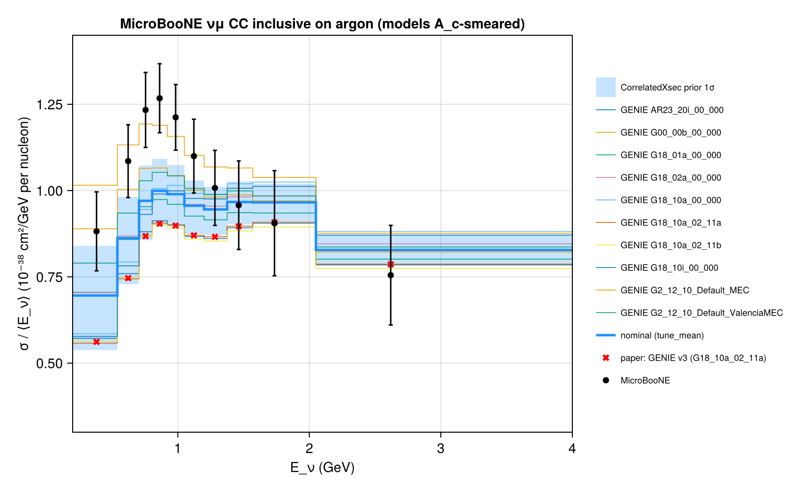
The νμ charged-current inclusive cross section per nucleon of argon as a function of the neutrino energy, 0.2–4 GeV, unfolded with the Wiener-SVD method (HEPData: σ, covariance, additional smearing matrix A_c), compared with the cross sections carried by Newtrinos.jl (module xsec): the ten GENIE tunes of generator_sigma on ⁴⁰Ar and the nominal model of CorrelatedXsec (the mean of the tunes) with its prior 1σ band. As in the paper, each model is averaged over the true-energy bins with the nominal BNB flux and smeared with A_c. The paper's "GENIE v3.00.06" is G18_10a_02_11a, one of the tunes: the Newtrinos chain reproduces the paper's (digitised) curve for it to 0.1 % in nine bins (0.7 % in the lowest) and its χ²: 19.1 vs 18.8 for 10 bins. The nominal model gives χ² = 11.3 (8.3 with its prior covariance); the tunes give 8.2–19.3 (GENIE 2.12 and G00_00b, with the largest low-energy cross sections, fit best), and the paper finds 8.6 for NEUT, 6.5 for GiBUU and 8.0 for its tuned GENIE.
Figures
νμ CC σ/⟨Eν⟩ on argon: MicroBooNE vs the A_c-smeared GENIE tunes and CorrelatedXsec nominal with its prior 1σ band, and the paper's GENIE v3 curve · Fig. 3a
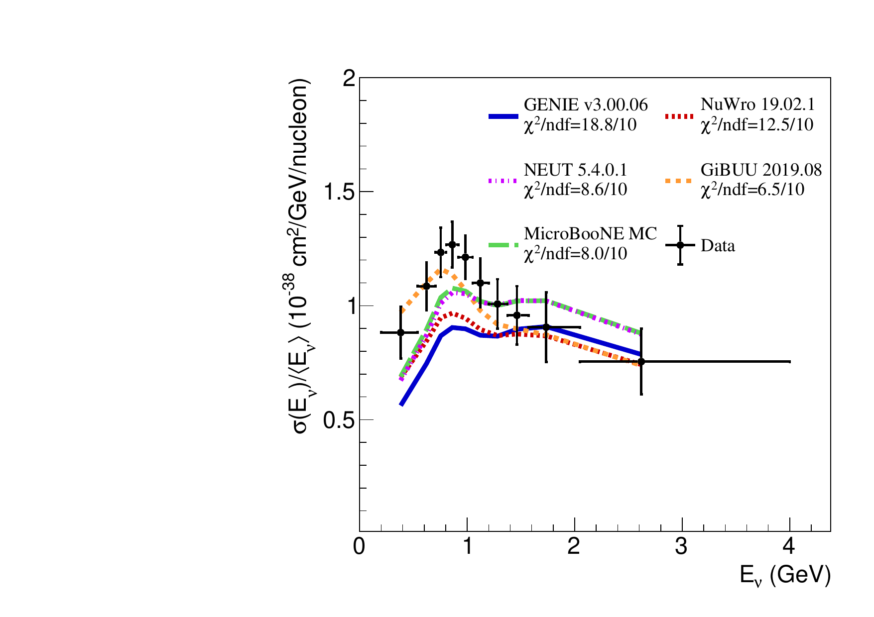
Original figure: MicroBooNE, Phys. Rev. Lett. 128, 151801 (2022), Fig. 3a, doi:10.1103/PhysRevLett.128.151801. Not our work; shown for comparison, all rights with the authors and publisher.
Known limitations
- The covariance has several near-zero eigenvalues (a property of the Wiener filter), so χ² is sensitive at the O(1) level to 10⁻³-level differences in binning or flux averaging. The published flux reproduces the quoted flux-weighted bin centres to 0.001 GeV except in the first and the last two bins (2.676 vs 2.619 GeV in 2.05–4 GeV), so the flux used in the analysis differed slightly.
- The paper's model curves are not tabulated; they were digitised from the vector figure (precision ≈ 0.1 %). Recomputing their χ² with the published covariance gives 0.4–0.9 more than quoted (19.2 vs 18.8 for GENIE v3), from that sensitivity.
- Below ~1.5 GeV the tunes differ by up to 40 % on argon; the data lie at the upper end. G18_10a_02_11a, the paper's GENIE v3, is at the low end (20–30 % below the data at 0.5–1.3 GeV); the nominal (mean of the tunes) is closer, and its prior band, from the tune spread and the physics knobs, covers most of the data.
- Model cross sections per nucleon of ⁴⁰Ar (σ per nucleus / 40), as the paper.
Reproduce
git clone https://github.com/Newtrinos-org/Newtrinos.jl.git && cd Newtrinos.jl && git checkout 78e71c310b- Download reproduce.jl and the
data/folder of this entry into an empty directory. julia -t 8 --project=/path/to/Newtrinos.jl reproduce.jl
# MicroBooNE νμ CC inclusive σ(Eν) on argon, 0.2–4 GeV (PRL 128, 151801 (2022); HEPData ins1954078 / arXiv ancillary
# files: unfolded σ, covariance and the additional smearing matrix A_c, in data/), compared with the cross sections of
# Newtrinos.jl (module `xsec`): the GENIE tunes (`generator_sigma`, ⁴⁰Ar per nucleon) and the reference model of
# `CorrelatedXsec` with its prior 1σ band. Following the paper, each model is averaged in the true-energy bins with the
# nominal BNB νμ flux at MicroBooNE (data/flux_bnb_numu_uboone.csv, from arXiv:1905.09694) and smeared with A_c
# (σ_smeared = A_c σ_model) before it is compared with the data. The paper's "GENIE v3.00.06" is G18_10a_02_11a, the
# reference tune here, which tests the chain against the paper's own curve (digitised, data/models_smeared_digitized.csv)
# and χ² (18.8 for 10 bins).
# Run from this directory with the Newtrinos.jl environment at the pinned commit:
#   julia --project=<path to Newtrinos.jl> reproduce.jl
using Newtrinos, CairoMakie, CSV, DataFrames, Printf, Statistics, Random, Distributions, LinearAlgebra

cd(@__DIR__); mkpath("ours"); mkpath("results")
const X = Newtrinos.xsec

readc(f) = CSV.read(f, DataFrame; comment = "#")
D = readc("data/sigma.csv")
C = Matrix{Float64}(CSV.read("data/covariance.csv", DataFrame; comment = "#", header = false))
Ac = Matrix{Float64}(CSV.read("data/Ac.csv", DataFrame; comment = "#", header = false))
paper = readc("data/models_smeared_digitized.csv")
flux = readc("data/flux_bnb_numu_uboone.csv")
edges = vcat(D.E_lo, D.E_hi[end])

# flux-weighted bin average ∫Φσ dE / ∫Φ dE on a fine grid (flux constant within its 50 MeV bins)
Ef = collect(range(0.2, 4.0, length = 3801))
Φ = [flux.flux[clamp(searchsortedlast(flux.E_lo, e), 1, nrow(flux))] for e in Ef]
binidx = [clamp(searchsortedlast(edges, e), 1, nrow(D)) for e in Ef]
fluxavg(σ) = [sum(Φ[binidx .== j] .* σ[binidx .== j]) / sum(Φ[binidx .== j]) for j in 1:nrow(D)]
@printf("flux-weighted bin centres: %s (paper %s)\n", round.(fluxavg(Ef), digits = 3), D.E_center)

tab = X.load_table()
at(v, e) = X.at_energies(tab.E, v, e)
TUNES = Symbol.(sort(tab.tunes))
σ_tune(t, e) = at(sum(X.generator_sigma(t, :Ar, :numu, false, :CC)), e) .* e     # σ per nucleon (σ/E × E)

xs = X.configure(X.CorrelatedXsec())
ref = xs.cfg.reference
sigf = xs.sigma(Ef; flavour = :numu, anti = false, current = :CC, target = :Ar)
model(p) = Ac * fluxavg(sigf(p) .* Ef)
rng = MersenneTwister(1)
draw() = map(p -> p isa Distribution ? rand(rng, p) : p, xs.priors)
samples = [draw() for _ in 1:500]
p0 = xs.params
M = reduce(hcat, [model(p) for p in samples])
Ccov = cov(M, dims = 2)

chi2(m, Cm = C) = (r = D.sigma .- m; dot(r, Cm \ r))
rows = [(model = "$(ref) (nominal)", chi2 = chi2(model(p0)), chi2_with_prior = chi2(model(p0), C + Ccov))]
smeared = Dict(t => Ac * fluxavg(σ_tune(t, Ef)) for t in TUNES)
for t in TUNES
    push!(rows, (model = string(t), chi2 = chi2(smeared[t]), chi2_with_prior = NaN))
end
for c in names(paper)[4:end]
    push!(rows, (model = "paper: $(c) (digitised)", chi2 = chi2(paper[!, c]), chi2_with_prior = NaN))
end
out = DataFrame(rows); out.ndf .= nrow(D)
CSV.write("results/chi2.csv", out)
CSV.write("results/smeared.csv", DataFrame(E_lo = D.E_lo, E_hi = D.E_hi, data = D.sigma, err = D.err,
                                           reference = round.(model(p0), digits = 4), prior_1sigma = round.(sqrt.(diag(Ccov)), digits = 4),
                                           paper_GENIE_v3 = paper[!, "GENIE_v3.00.06"]))
show(stdout, out, allrows = true, allcols = true); println()

# figure: σ/⟨E⟩ per bin as in the paper (data, smeared models)
Ec = D.E_center
fig = Figure(size = (820, 500))
ax = Axis(fig[1, 1], xlabel = "E_ν (GeV)", ylabel = "σ / ⟨E_ν⟩ (10⁻³⁸ cm²/GeV per nucleon)", limits = (0.2, 4.0, 0.3, 1.45),
          title = "MicroBooNE νμ CC inclusive on argon (models A_c-smeared)")
stairs_ = (y) -> (vcat(edges[1], repeat(edges[2:end-1], inner = 2), edges[end]), repeat(y, inner = 2))
lo, hi = [quantile(r, 0.16) for r in eachrow(M)], [quantile(r, 0.84) for r in eachrow(M)]
band!(ax, stairs_(lo ./ Ec)[1], stairs_(lo ./ Ec)[2], stairs_(hi ./ Ec)[2], color = (:dodgerblue, 0.25), label = "CorrelatedXsec prior 1σ")
for (i, t) in enumerate(TUNES)
    lines!(ax, stairs_(smeared[t] ./ Ec)..., color = (Makie.wong_colors()[mod1(i, 7)], 0.8), linewidth = 1, label = "GENIE $(t)")
end
lines!(ax, stairs_(model(p0) ./ Ec)..., color = :dodgerblue, linewidth = 2.5, label = "nominal ($(ref))")
scatter!(ax, Ec, paper[!, "GENIE_v3.00.06"] ./ Ec, marker = :xcross, color = :red, markersize = 10, label = "paper: GENIE v3 (G18_10a_02_11a)")
errorbars!(ax, Ec, D.sigma ./ Ec, D.err ./ Ec, color = :black, whiskerwidth = 4)
scatter!(ax, Ec, D.sigma ./ Ec, color = :black, label = "MicroBooNE")
Legend(fig[1, 2], ax, framevisible = false, labelsize = 9)
save("ours/sigma_enu.png", fig)
Provenance
| Newtrinos.jl commit | 78e71c310b (xsec (generator_sigma, CorrelatedXsec)) |
|---|---|
| Run date | 2026-10-12T12:21:16Z |
| Wall time | 1.4 min (4 threads) |
| Julia | 1.12.5 |
| Machine | AMD EPYC 7702P 64-Core Processor, 128 hardware threads, Linux |
| Environment | newtrinos_Manifest.toml · run.toml |
Downloads
CSV files hold one row per scan point: the scanned and profiled parameters
(sin2_theta23, dm2_32 in eV², dcp in rad, nuisance parameters), dchi2 = −2Δ log L
and the log-likelihood. JLD2 files contain the full NewtrinosResult objects.
| File | Size | SHA-256 |
|---|---|---|
| ours/sigma_enu.png | 139.6 kB | 42722114f6cc… |
| results/chi2.csv | 810 B | b06ba7f62054… |
| results/smeared.csv | 501 B | f0a12e8e45b1… |