
COHERENT · Phys. Rev. Lett. 129, 081801 (2022)
Measurement of the Coherent Elastic Neutrino-Nucleus Scattering Cross Section on CsI by COHERENT
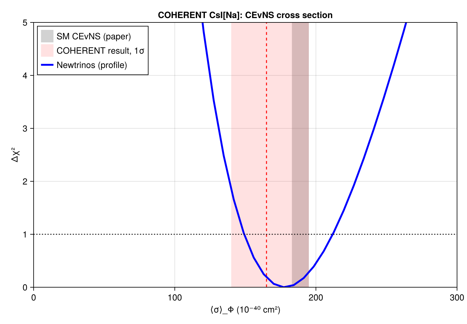
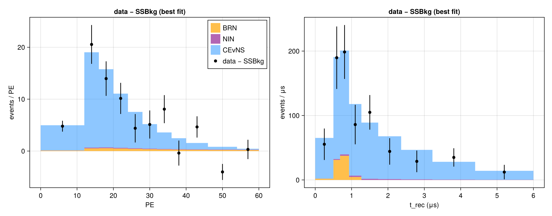
Flux-averaged CEvNS cross section on CsI[Na] from the full COHERENT CsI data set, fitted in recoil (PE) and time, with the SM-scaled cross-section model (σ = scale × σ_SM) and all background and detector nuisances profiled, following the release's prescription (PE < 60, t_rec < 6 μs; flux normalised to 3.198×10²³ POT and 0.0848 ν per flavour per proton; efficiency applied within the PE bins; steady-state background from the AC PE distribution with an exponential time dependence). The best fit reproduces the paper's Table I: 314.5 CEvNS events (COHERENT 306 ± 20), 1275.5 steady-state background (1273 ± 24), 17.5 BRN (17.3 ± 4.5) and 5.1 NIN (5.5 ± 2.0), with the threshold (efficiency) nuisance pulled by 0.48σ (paper: 0.4σ); the Newtrinos SM prediction is 323.5 events at the nominal nuisance parameters and 334 at the best-fit ones (paper 341 ± 11 ± 42) and the cross section ≈ 178 [150, 212] × 10⁻⁴⁰ cm² (paper 165 +30 −25).
Figures
Δχ² vs flux-averaged CEvNS cross section · Suppl. Fig. 4
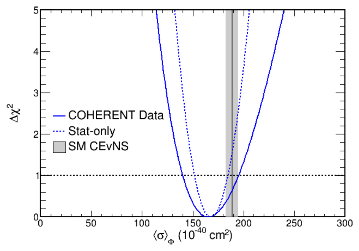
Original figure: COHERENT, Phys. Rev. Lett. 129, 081801 (2022), Suppl. Fig. 4, doi:10.1103/PhysRevLett.129.081801. Not our work; shown for comparison, all rights with the authors and publisher.
Data residual over the steady-state background vs best-fit CEvNS, BRN and NIN, projected onto PE and t_rec · Fig. 3
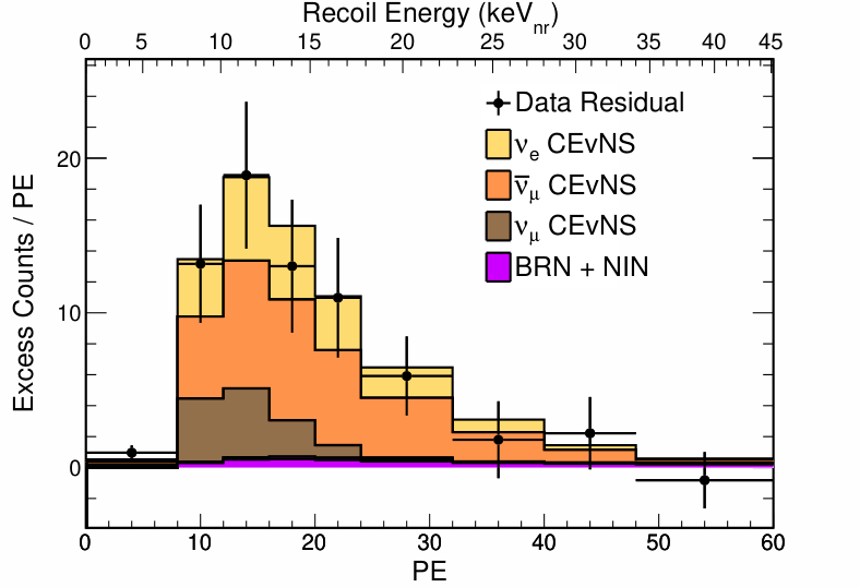
Original figure: COHERENT, Phys. Rev. Lett. 129, 081801 (2022), Fig. 3, doi:10.1103/PhysRevLett.129.081801. Not our work; shown for comparison, all rights with the authors and publisher.
Known limitations
- The x axis is scale × the paper's SM prediction ⟨σ⟩_Φ = 189 × 10⁻⁴⁰ cm²; the official curve is a raster image, so the paper's quoted result (165 +30 −25) × 10⁻⁴⁰ cm² is shown instead.
- sin²θ_W is fixed; the nuclear radii are constrained by their priors (form-factor uncertainty).
- Until Newtrinos 8d6b207 the module evaluated the efficiency at the PE bin centres (no signal in 8–12 PE), scaled the flux tables as rates at 1.4 MW (1.33× too many neutrinos), fitted up to 196 PE and used the raw 2D AC histogram as steady-state background; this gave 260 CEvNS events and a cross section of ≈ 134 × 10⁻⁴⁰ cm².
- The cross-section axis is scale × 189 × 10⁻⁴⁰ cm² (the paper's SM value); the Newtrinos SM rate is 5 % below the paper's (323.5 vs 341 events), partly from the 0.5 MeV energy offset of the flux tables (see the SNS flux entry) and the isotope fractions.
Reproduce
git clone https://github.com/Newtrinos-org/Newtrinos.jl.git && cd Newtrinos.jl && git checkout 8d6b207a1d- Download reproduce.jl into an empty directory.
julia -t 8 --project=/path/to/Newtrinos.jl reproduce.jl
# Reproduction of COHERENT, Phys. Rev. Lett. 129, 081801 (2022) [arXiv:2110.07730] with Newtrinos.jl (module `coherent_csi`, SM-scaled cross-section model).
# Data: COHERENT CsI[Na] full data set release (supplemental material of the paper).
# Run from this directory with the Newtrinos.jl environment at the pinned commit:
#   julia -t 8 --project=<path to Newtrinos.jl> reproduce.jl
using Newtrinos, Distributions, DataStructures, Accessors, FileIO, CairoMakie, CSV, DataFrames, DensityInterface

cd(@__DIR__); mkpath("ours"); mkpath("results"); mkpath("cache")

# CSV export of a profile scan: one row per grid point, ASCII column names, oscillation parameters in physical
# units (sin²θ, Δm²₃₂ = Δm²₃₁ − Δm²₂₁ in eV², δCP in rad), dchi2 = -2Δlog L w.r.t. `ref` (default: the scan's best fit)
function save_csv(path, r; ref = maximum(r.values.log_posterior))
    ascii(k) = replace(string(k), "θ" => "theta", "Δm²" => "dm2_", "δ" => "d", "₁" => "1", "₂" => "2", "₃" => "3", "CP" => "cp")
    cols = OrderedDict{String,Any}()
    for (k, v) in pairs(r.values)
        x = vec(v)
        if startswith(string(k), "θ")
            cols["sin2_" * ascii(k)] = sin.(x) .^ 2
        elseif k == :Δm²₃₁
            cols["dm2_32"] = x .- vec(r.values.Δm²₂₁)
        end
        cols[ascii(k)] = x
    end
    cols["dchi2"] = 2 .* (ref .- vec(r.values.log_posterior))
    haskey(cols, "llh") && (cols["log_likelihood"] = pop!(cols, "llh"))
    first_cols = filter(in(keys(cols)), ["sin2_theta23", "dm2_32", "dcp", "dchi2", "log_likelihood", "log_posterior"])
    CSV.write(path, DataFrame(cols)[:, vcat(first_cols, setdiff(collect(keys(cols)), first_cols))])
end

experiments = (coherent_csi = Newtrinos.coherent_csi.configure(xsec_model = :sm_scale),)
likelihood = Newtrinos.generate_likelihood(experiments)
p = Newtrinos.get_params(experiments)
priors = Newtrinos.get_priors(experiments)

# the CEvNS cross section is scaled as a whole (cevns_xsec_scale = σ / σ_SM); sin²θ_W fixed at its default,
# nuclear radii constrained by their priors (form-factor uncertainty), all background and detector nuisances profiled
priors = merge(priors, (sin2thetaW = p.sin2thetaW, cevns_xsec_scale = Uniform(0.3, 1.8)))
mkpath("cache/scale")
result = Newtrinos.profile(likelihood, priors, OrderedDict(:cevns_xsec_scale => 41), p, cache_dir = "cache/scale")
FileIO.save("results/coherent_csi.jld2", Dict("scale" => result))
save_csv("results/coherent_csi_scale.csv", result)

# supplemental Fig. 4: Δχ² vs flux-averaged cross section; x = scale × σ_SM with the paper's
# SM prediction ⟨σ⟩_Φ = (189 ± 6) × 10⁻⁴⁰ cm², result (165 +30 −25) × 10⁻⁴⁰ cm²
σSM = 189.0
x = result.axes.cevns_xsec_scale .* σSM
dχ² = 2 .* (maximum(result.values.log_posterior) .- result.values.log_posterior)
fig = Figure(size = (750, 520))
ax = Axis(fig[1, 1], title = "COHERENT CsI[Na]: CEvNS cross section", xlabel = "⟨σ⟩_Φ (10⁻⁴⁰ cm²)", ylabel = "Δχ²")
vspan!(ax, [σSM - 6], [σSM + 6], color = (:gray, 0.35), label = "SM CEvNS (paper)")
vspan!(ax, [165 - 25], [165 + 30], color = (:red, 0.12), label = "COHERENT result, 1σ")
vlines!(ax, [165], color = :red, linestyle = :dash)
lines!(ax, x, dχ², color = :blue, linewidth = 3, label = "Newtrinos (profile)")
hlines!(ax, [1.0], color = :black, linestyle = :dot)
xlims!(ax, 0, 300); ylims!(ax, 0, 5)
axislegend(ax, position = :lt)
save("ours/supp_fig4_dchi2_xsec.png", fig)

# Fig. 3: data residual over the steady-state background compared with the best-fit CEvNS, BRN and NIN predictions,
# projected onto PE and t_rec
using BAT: distprod
const CSI = Newtrinos.coherent_csi
e = experiments.coherent_csi; a = e.assets
bf = Newtrinos.find_mle(likelihood, distprod(; merge(priors, (cevns_xsec_scale = Uniform(0.3, 1.8),))...), p)[3]
sig = CSI.get_expected(bf, e.physics, a); brn, nin, ss = CSI.get_backgrounds(bf, a)
sig_sm = CSI.get_expected(merge(bf, (cevns_xsec_scale = 1.0,)), e.physics, a)
N = a.observed
open("results/summary.txt", "w") do io
    println(io, "events in PE < 60, t < 6 μs (Newtrinos best fit | COHERENT Table I best fit)")
    println(io, "CEvNS   $(round(sum(sig), digits = 1)) | 306 ± 20   (Newtrinos SM prediction $(round(sum(sig_sm), digits = 1)); COHERENT 341 ± 11 ± 42)")
    println(io, "SSBkg   $(round(sum(ss), digits = 1)) | 1273 ± 24")
    println(io, "BRN     $(round(sum(brn), digits = 1)) | 17.3 ± 4.5")
    println(io, "NIN     $(round(sum(nin), digits = 1)) | 5.5 ± 2.0")
    println(io, "cross-section scale (σ / σ_SM,Newtrinos) $(round(bf.cevns_xsec_scale, digits = 3)); efficiency pull $(round(bf.coherent_csi_eff_sigma, digits = 2)) σ; flux onset $(round(bf.flux_onset, digits = 1)) ns")
end
print(read("results/summary.txt", String))
fig = Figure(size = (1150, 450))
for (col, (dim, edges, xl)) in enumerate(((2, a.out_edges, "PE"), (1, a.time_edges ./ 1e3, "t_rec (μs)")))
    proj(h) = vec(sum(h, dims = dim))
    w = diff(edges); c = 0.5 .* (edges[1:end-1] .+ edges[2:end])
    local ax = Axis(fig[1, col], xlabel = xl, ylabel = col == 1 ? "events / PE" : "events / μs", title = "data − SSBkg (best fit)")
    stk = (brn = proj(brn), nin = proj(nin), sig = proj(sig))
    band!(ax, repeat(edges, inner = 2)[2:end-1], zeros(2 * length(w)), repeat(stk.brn ./ w, inner = 2), color = (:orange, 0.7), label = "BRN")
    band!(ax, repeat(edges, inner = 2)[2:end-1], repeat(stk.brn ./ w, inner = 2), repeat((stk.brn .+ stk.nin) ./ w, inner = 2), color = (:purple, 0.6), label = "NIN")
    band!(ax, repeat(edges, inner = 2)[2:end-1], repeat((stk.brn .+ stk.nin) ./ w, inner = 2), repeat((stk.brn .+ stk.nin .+ stk.sig) ./ w, inner = 2),
          color = (:dodgerblue, 0.5), label = "CEvNS")
    r = proj(N) .- proj(ss)
    errorbars!(ax, c, r ./ w, sqrt.(proj(N)) ./ w, color = :black); scatter!(ax, c, r ./ w, color = :black, label = "data − SSBkg")
    col == 1 && axislegend(ax, position = :rt)
end
save("ours/fig3_residuals.png", fig)
Provenance
| Newtrinos.jl commit | 8d6b207a1d (coherent_csi, cevns_xsec (xsec_model = :sm_scale), sns_flux) |
|---|---|
| Run date | 2026-10-11T11:39:27Z |
| Wall time | 3.0 min (8 threads) |
| Julia | 1.12.5 |
| Machine | AMD EPYC 7702P 64-Core Processor, 128 hardware threads, Linux |
| Environment | newtrinos_Manifest.toml · run.toml |
Downloads
CSV files hold one row per scan point: the scanned and profiled parameters
(sin2_theta23, dm2_32 in eV², dcp in rad, nuisance parameters), dchi2 = −2Δ log L
and the log-likelihood. JLD2 files contain the full NewtrinosResult objects.
| File | Size | SHA-256 |
|---|---|---|
| ours/fig3_residuals.png | 81.3 kB | 0571c5f0dc78… |
| ours/supp_fig4_dchi2_xsec.png | 89.0 kB | b93b552d8802… |
| results/coherent_csi.jld2 | 33.9 kB | 7499a2be951d… |
| results/coherent_csi_scale.csv | 10.7 kB | 3bc7ceafa013… |
| results/summary.txt | 338 B | df312e4b308e… |