
Borexino · Phys. Rev. Lett. 129, 252701 (2022)
Improved Measurement of Solar Neutrinos from the Carbon-Nitrogen-Oxygen Cycle by Borexino and Its Implications for the Standard Solar Model
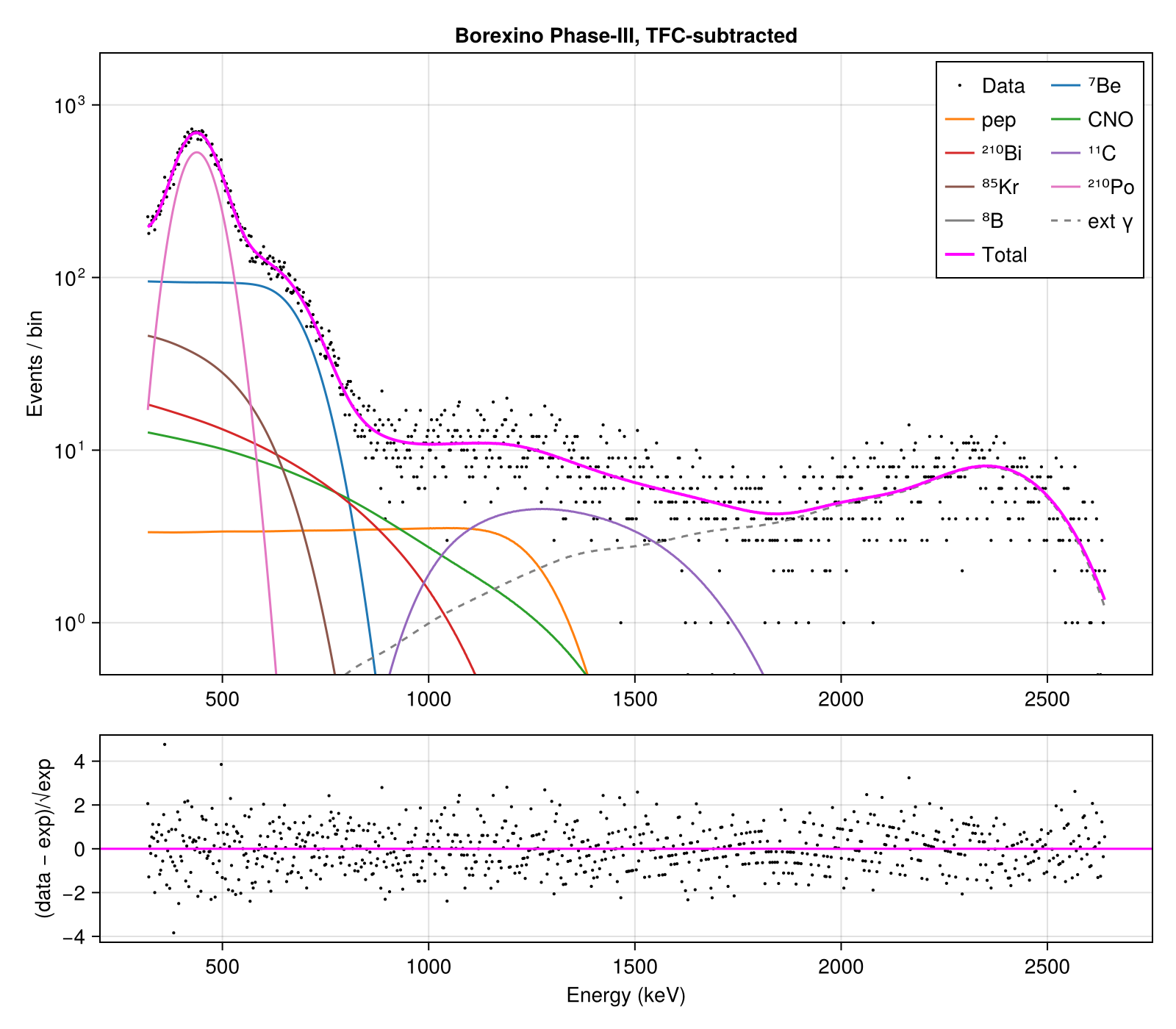
CNO-ν interaction rate from the Borexino Phase-III TFC-subtracted energy spectrum (Jan 2017 – Oct 2021, 1431.6 d × 71.3 t, 817 bins from the Borexino open data). Newtrinos fits the spectrum with the Borexino Monte Carlo spectral shapes, the solar rates predicted by its solar-flux, oscillation and ν–e scattering modules, free background rates, an energy response calibrated on Borexino's best-fit spectrum and the ²¹⁰Bi upper limit (10.8 ± 1.0 cpd/100 t). Borexino finds 6.7 (+2.0/−0.8) cpd/100 t (6.6 +2.0/−0.7 statistical only); Newtrinos finds 6.80 (+1.83/−1.59) with the priors that stand in for the TFC-tagged spectrum and radial distribution (module default) and 6.98 (+3.03/−2.22) with these backgrounds left free (intervals from −2Δln L = 1). The profile with priors follows the published one between 0.5 and 12 cpd/100 t.
Figures
CNO-ν rate likelihood profile · Fig. 2(b)
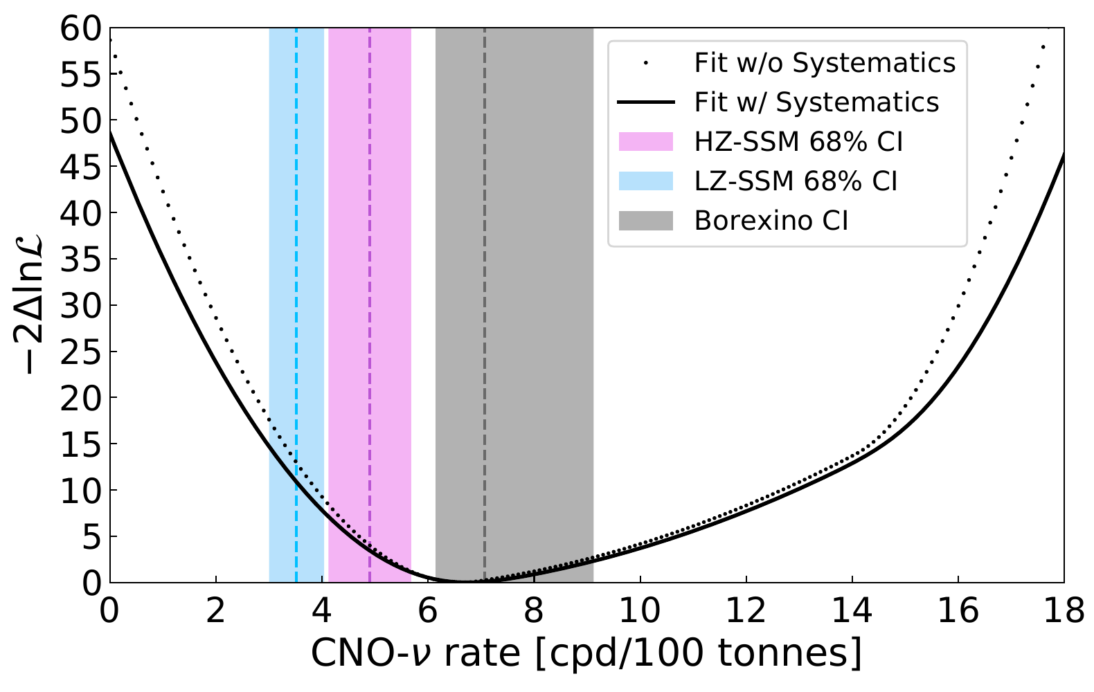
Original figure: Borexino, Phys. Rev. Lett. 129, 252701 (2022), Fig. 2(b), doi:10.1103/PhysRevLett.129.252701. Not our work; shown for comparison, all rights with the authors and publisher.
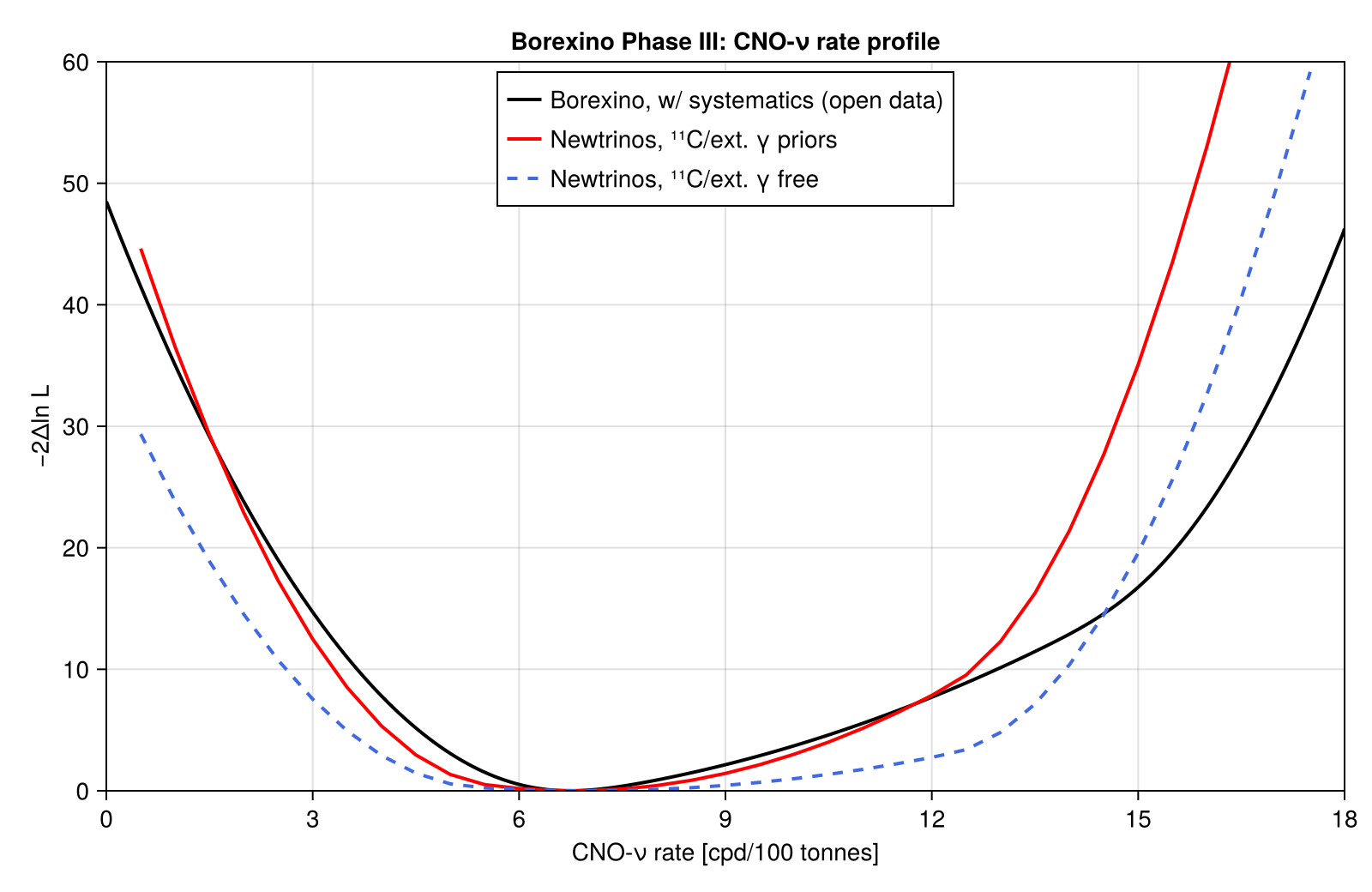
TFC-subtracted energy spectrum and best fit · Fig. 2(a)
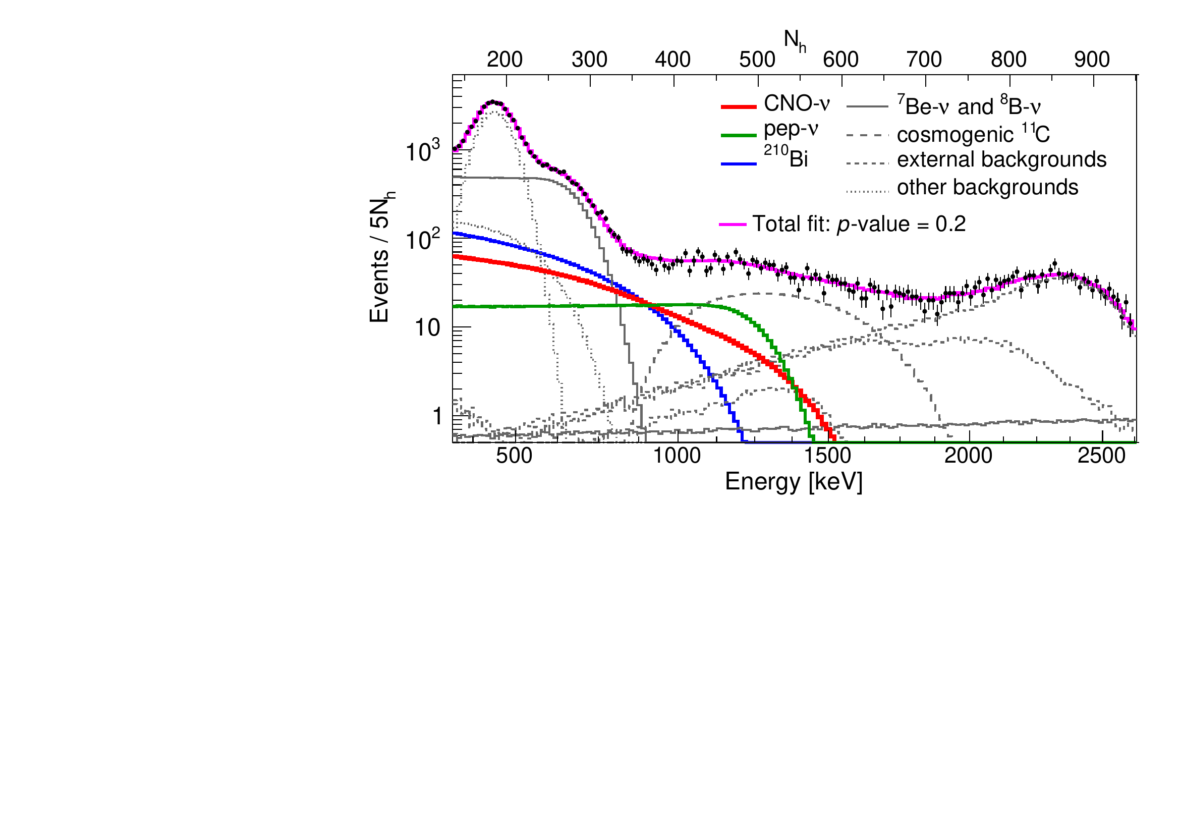
Original figure: Borexino, Phys. Rev. Lett. 129, 252701 (2022), Fig. 2(a), doi:10.1103/PhysRevLett.129.252701. Not our work; shown for comparison, all rights with the authors and publisher.
Known limitations
- Borexino fits the TFC-subtracted and TFC-tagged spectra and the radial distribution simultaneously; only the TFC-subtracted spectrum is public. Gaussian priors (3 %) on ¹¹C and the external γ rates around their values in Borexino's best fit stand in for the missing information; without them (dashed curve) the CNO constraint is weaker.
- The energy response of the public Monte Carlo shapes (from the sensitivity study arXiv:2005.12829) is mapped to the data with a scale, offset and extra smearing calibrated on Borexino's best-fit spectrum, with nuisance parameters; Borexino's systematic uncertainties (non-linearity, non-uniformity, ²¹⁰Bi shape) are not modelled otherwise.
- The fit is binned in keV as published; Borexino fits in the N_h energy estimator.
- The ⁸B spectrum is not among the public shapes and is computed from the ν–e response with Gaussian resolution; cosmogenic ⁶He and ¹⁰C are not included.
- pep is constrained by the B23 solar-model prior (≈1 %) instead of Borexino's 2.74 ± 0.04 cpd/100 t; the oscillation parameters are at the Newtrinos defaults.
- The published profile includes systematic uncertainties; the statistical-only profile of the original figure is not available as data.
- Above ≈13 cpd/100 t the Newtrinos profile rises faster than the published one (−2Δln L > 10, beyond the region relevant for fits).
Reproduce
git clone https://github.com/Newtrinos-org/Newtrinos.jl.git && cd Newtrinos.jl && git checkout c6612c255a- Download reproduce.jl into an empty directory.
julia -t 8 --project=/path/to/Newtrinos.jl reproduce.jl
# Reproduction of Borexino, Phys. Rev. Lett. 129, 252701 (2022) [arXiv:2205.15975]: CNO-ν rate from the
# Phase-III TFC-subtracted spectrum (Fig. 2a) and its likelihood profile (Fig. 2b), with Newtrinos.jl.
# Run from this directory with the Newtrinos.jl environment at the pinned commit:
#   julia -t 16 --project=<path to Newtrinos.jl> reproduce.jl
using Newtrinos, Distributions, DensityInterface, Optim, ADTypes, ForwardDiff, CairoMakie, DelimitedFiles, Printf, CSV, DataFrames

cd(@__DIR__); mkpath("ours"); mkpath("results")
const B = Newtrinos.borexino_ph3
# scalar flux normalisations (solar_norm_*), so that ⁷Be, CNO and pep can be treated individually
physics = merge(B.default_physics(), (solar_flux = Newtrinos.solar_flux.configure(
    Newtrinos.solar_flux.SolarFluxConfig(systematics = Newtrinos.solar_flux.SSMPriors())),))
published = readdlm(joinpath(B.DATADIR, "Phase3Final_BiULLarge_Golden_Energy_Radial_May18_HybridMethod.txt"))

# Borexino conditions: ⁷Be and CNO rates free, pep at the SSM (B23 prior, ~1 %; Borexino: 2.74 ± 0.04 cpd/100 t),
# ⁸B fixed; oscillation parameters, pp and hep at the Newtrinos defaults. The CNO components ¹³N, ¹⁵O, ¹⁷F share one
# normalisation. All Borexino nuisances (backgrounds, energy response) are profiled with their module priors.
function fitter(background_priors)
    bx = B.configure(physics; background_priors)
    exps = (borexino_ph3 = bx,)
    llh = Newtrinos.generate_likelihood(exps)
    p0 = Newtrinos.get_params(exps)
    priors = Newtrinos.get_priors(exps)
    nuis = vcat(collect(keys(bx.params)), [:solar_norm_pep])
    toparams(be7, cno, y) = merge(p0, (solar_norm_be7 = be7, solar_norm_n13 = cno, solar_norm_o15 = cno, solar_norm_f17 = cno),
                                  NamedTuple{Tuple(nuis)}(Tuple(y)))
    nlp(be7, cno, y) = -(logdensityof(llh, toparams(be7, cno, y)) + sum(logpdf(priors[k], y[i]) for (i, k) in enumerate(nuis)))
    lo = vcat(0.3, [minimum(priors[k]) for k in nuis]); hi = vcat(2.0, [maximum(priors[k]) for k in nuis])
    y0 = vcat(1.0, [p0[k] for k in nuis])
    function minimise(f, x0, lo, hi)
        r = optimize(f, lo, hi, clamp.(x0, lo .+ 1e-6, hi .- 1e-6), Fminbox(LBFGS()),
                     Optim.Options(iterations=500, outer_iterations=10, g_tol=1e-5); autodiff=ADTypes.AutoForwardDiff())
        Optim.minimizer(r), Optim.minimum(r)
    end
    # global best fit (CNO normalisation free in [0, 4])
    xb, mb = minimise(x -> nlp(x[1], x[2], x[3:end]), vcat(1.0, 1.0, y0[2:end]), vcat(lo[1], 0.0, lo[2:end]), vcat(hi[1], 4.0, hi[2:end]))
    pb = toparams(xb[1], xb[2], xb[3:end])
    rates = B.solar_rates(pb, bx.physics, bx.assets)
    per_norm = rates.cno / xb[2]                      # CNO rate [cpd/100 t] per unit normalisation
    # profile in the CNO rate
    profile(cno) = 2 * (minimise(y -> nlp(y[1], cno / per_norm, y[2:end]), vcat(xb[1], xb[3:end]), lo, hi)[2] - mb)
    (; bx, pb, rates, nuis, xb, profile)
end

grid = collect(0.5:0.5:17.5)
summary = IOBuffer()
fits = Dict{Symbol, Any}()
for bp in (:constrained, :free)
    f = fitter(bp)
    prof = zeros(length(grid))
    Threads.@threads for i in eachindex(grid)
        prof[i] = f.profile(grid[i])
    end
    fits[bp] = (; f..., prof)
    CSV.write("results/cno_profile_$(bp).csv", DataFrame(cno_rate_cpd100t = grid, minus2_dlnL = prof))
    # 68 % interval from −2Δln L = 1 (linear interpolation)
    cross(xs, ys) = xs[1] + (1 - ys[1]) * (xs[2] - xs[1]) / (ys[2] - ys[1])
    g = vcat(grid, f.rates.cno); p = vcat(prof, 0.0); o = sortperm(g); g, p = g[o], p[o]
    ib = findfirst(==(0.0), p)
    il = findfirst(<(1), p[1:ib]); iu = ib - 1 + findfirst(>(1), p[ib:end])
    lo1 = il > 1 ? cross(g[il-1:il], p[il-1:il]) : NaN
    up1 = cross(g[iu-1:iu], p[iu-1:iu])
    println(summary, @sprintf("[%s] best fit: CNO = %.2f (+%.2f/−%.2f, −2ΔlnL = 1) cpd/100 t, ⁷Be = %.2f, pep = %.3f cpd/100 t",
                              bp, f.rates.cno, up1 - f.rates.cno, f.rates.cno - lo1, f.rates.be7, f.rates.pep))
    println(summary, "    nuisances: ", join([@sprintf("%s=%.3g", replace(string(k), "borexino_ph3_" => ""), v) for (k, v) in zip(f.nuis, f.xb[3:end])], " "))
end
println(summary, "Borexino (PRL 129, 252701): CNO = 6.7 +2.0/−0.8 cpd/100 t (6.6 +2.0/−0.7 statistical only)")
summary_text = String(take!(summary)); write("results/summary.txt", summary_text); print(summary_text)

# Fig. 2b: CNO profile
fig = Figure(size=(800, 520))
ax = Axis(fig[1, 1], xlabel="CNO-ν rate [cpd/100 tonnes]", ylabel="−2Δln L", title="Borexino Phase III: CNO-ν rate profile")
lines!(ax, published[:, 1], published[:, 3], color=:black, linewidth=2, label="Borexino, w/ systematics (open data)")
for (bp, col, lab) in ((:constrained, :red, "Newtrinos, ¹¹C/ext. γ priors"), (:free, :royalblue, "Newtrinos, ¹¹C/ext. γ free"))
    f = fits[bp]; g = vcat(grid, f.rates.cno); p = vcat(f.prof, 0.0); o = sortperm(g)
    lines!(ax, g[o], p[o], color=col, linewidth=2, linestyle=(bp == :free ? :dash : :solid), label=lab)
end
xlims!(ax, 0, 18); ylims!(ax, 0, 60); axislegend(ax, position=:ct)
save("ours/fig2b_cno_profile.png", fig)

# Fig. 2a: spectrum at the best fit (with priors)
f = fits[:constrained]
save("ours/fig2a_spectrum.png", f.bx.plot(f.pb))
Provenance
| Newtrinos.jl commit | c6612c255a (solar_flux, solar_xsec, solar_common, borexino_ph3) |
|---|---|
| Run date | 2026-10-21T17:04:06Z |
| Wall time | 13.1 min (128 threads) |
| Julia | 1.12.5 |
| Machine | AMD EPYC 7702P 64-Core Processor, 128 hardware threads, Linux |
| Environment | newtrinos_Manifest.toml · run.toml |
Downloads
CSV files hold one row per scan point: the scanned and profiled parameters
(sin2_theta23, dm2_32 in eV², dcp in rad, nuisance parameters), dchi2 = −2Δ log L
and the log-likelihood. JLD2 files contain the full NewtrinosResult objects.
| File | Size | SHA-256 |
|---|---|---|
| ours/fig2a_spectrum.png | 308.4 kB | a85db8e6d95a… |
| ours/fig2b_cno_profile.png | 152.0 kB | 45f83ae4ae0f… |
| results/cno_profile_constrained.csv | 837 B | 51f00c0b8d48… |
| results/cno_profile_free.csv | 843 B | 9cef3cd352df… |
| results/summary.txt | 670 B | 85de1a47ed2a… |