
J. A. Formaggio, G. P. Zeller · Rev. Mod. Phys. 84, 1307 (2012)
From eV to EeV: Neutrino Cross Sections Across Energy Scales
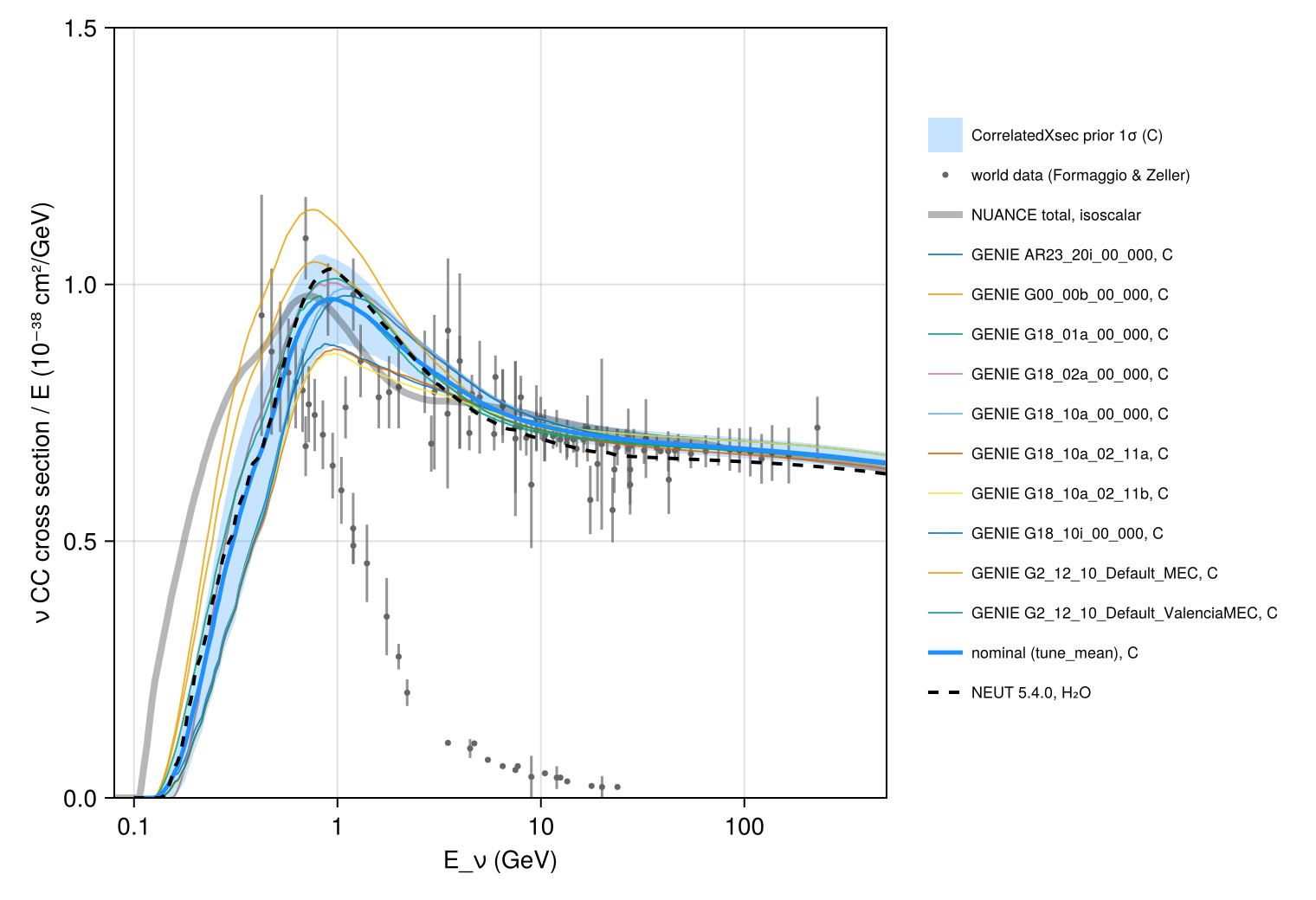
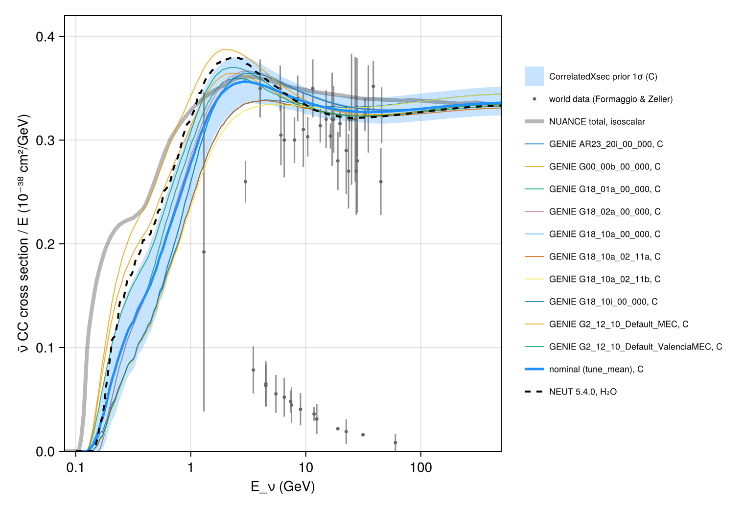
Total charged-current νμ and ν̄μ cross sections per nucleon divided by energy, from 0.1 to 500 GeV, as carried by Newtrinos.jl (module xsec): the per-process GENIE cross sections of ten tunes (generator_sigma, GENIE 2.12 to AR23_20i, on carbon, i.e. an isoscalar target as in the compilation), NEUT 5.4.0 on water, and the nominal model of CorrelatedXsec (the mean of the tunes) with its prior 1σ band, the cross-section model shared by all experiments in global fits. They are compared with the world data and the NUANCE prediction (total, and QE / RES / DIS) of the review's Fig. 15. Curves and data points are extracted from the vector figures of the arXiv source (data/extract_fz.py). In the deep-inelastic region (30–300 GeV) the prior 1σ bands are [0.662, 0.701] (νμ) and [0.319, 0.345] (ν̄μ) × 10⁻³⁸ cm²/GeV, against 0.677 and 0.323 for the extracted world data; the ten tunes span 0.669–0.695 and 0.326–0.337. Below 1 GeV the tunes differ by up to 60 %; the band (νμ: 0.62–0.90 at 0.5 GeV, 0.88–1.05 at 1 GeV) covers most of them.
Figures
νμ CC cross section per nucleon / E: world data, NUANCE, the GENIE tunes and NEUT, and the CorrelatedXsec nominal with its prior band · Fig. 15 (top)
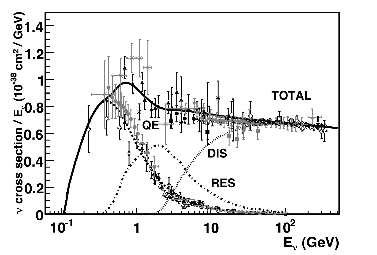
Original figure: J. A. Formaggio, G. P. Zeller, Rev. Mod. Phys. 84, 1307 (2012), Fig. 15 (top), doi:10.1103/RevModPhys.84.1307. Not our work; shown for comparison, all rights with the authors and publisher.
ν̄μ CC cross section per nucleon / E · Fig. 15 (bottom)
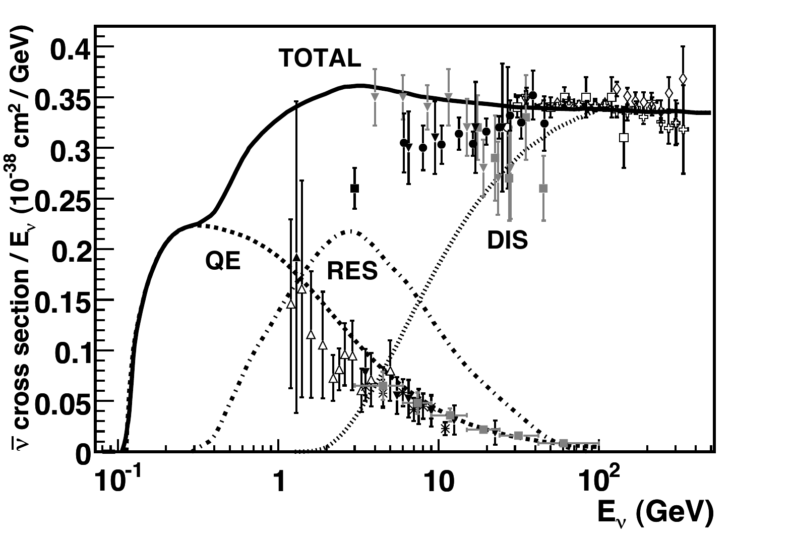
Original figure: J. A. Formaggio, G. P. Zeller, Rev. Mod. Phys. 84, 1307 (2012), Fig. 15 (bottom), doi:10.1103/RevModPhys.84.1307. Not our work; shown for comparison, all rights with the authors and publisher.
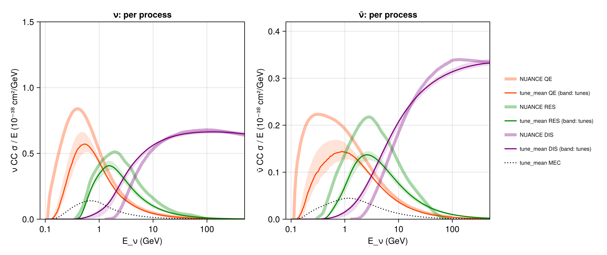
Per process (QE, RES, DIS; MEC): the nominal (mean of the tunes) and the spread of the tunes vs NUANCE · Fig. 15 (QE, RES, DIS curves)
Fig. 15 (QE, RES, DIS curves)
Known limitations
- GENIE curves are per nucleon of ¹²C (isoscalar); NEUT 5.4.0 is only available for water (digitised from T. Wester's Super-K thesis, valid up to 26 GeV and continued with the G18_10a_02_11a shape above), which makes it a few percent lower than isoscalar for neutrinos in the DIS region (0.654 vs 0.669–0.695).
- Below ~1 GeV the tunes differ strongly (νμ at 0.5 GeV: 0.63–1.04 × 10⁻³⁸ cm²/GeV): nuclear models (Fermi gas vs local Fermi gas / spectral function, RPA), M_A and MEC. The nominal (mean of the tunes) lies in the middle of this spread; its prior band (16–84 % of 500 draws) covers most tunes, while G18_10a_02_11a and AR23 are at the low end and GENIE 2.12 / G00_00b at the high end. The NUANCE total is higher still; the low-energy data in the figure are mostly QE-only measurements on other targets.
- Per process, definitions differ between generators: NUANCE's QE is per free nucleon (no nuclear suppression), GENIE's on carbon; GENIE's DIS includes the non-resonant low-W region; GENIE's MEC (2p2h) has no NUANCE counterpart. Only totals are directly comparable.
- The prior band is the 16–84 % range of 500 draws of all CorrelatedXsec parameters from their priors (PCA modes of the tune spread, M_A^QE, process normalisations, ν̄/ν); it describes the model uncertainty before any experiment constrains it.
- Data extraction: points are recovered from the marker shapes of the vector figure, with symmetric errors from the vertical bars. 109 νμ and 45 ν̄μ points are recovered, which is incomplete where markers overlap (the dense QE points at 1–3 GeV and most ν̄ points above 60 GeV).
Reproduce
git clone https://github.com/Newtrinos-org/Newtrinos.jl.git && cd Newtrinos.jl && git checkout 78e71c310b- Download reproduce.jl and the
data/folder of this entry into an empty directory. julia -t 8 --project=/path/to/Newtrinos.jl reproduce.jl
# Charged-current νμ / ν̄μ cross sections of Newtrinos.jl (module `xsec`) compared with the world data and the
# NUANCE prediction compiled by Formaggio & Zeller, Rev. Mod. Phys. 84, 1307 (2012), Fig. 15. The curves and data
# points are extracted from the vector figures of the arXiv source (data/extract_fz.py).
#
# Newtrinos curves: the per-process GENIE splines carried by `xsec` (`generator_sigma`, all tunes) on carbon
# (isoscalar, as the compilation), NEUT 5.4.0 on water (the only target it is available for), and the reference model
# of `CorrelatedXsec` with its prior 1σ band (all its parameters sampled from their priors).
# Run from this directory with the Newtrinos.jl environment at the pinned commit:
#   julia --project=<path to Newtrinos.jl> reproduce.jl
using Newtrinos, CairoMakie, CSV, DataFrames, Printf, Statistics, Random, Distributions

cd(@__DIR__); mkpath("ours"); mkpath("results")
const X = Newtrinos.xsec

E = 10 .^ range(-1, log10(500), length = 400)
tab = X.load_table()
at(v) = X.at_energies(tab.E, v, E)
TUNES = Symbol.(sort(tab.tunes))
σ_tune(t, anti; target = :C) = at(sum(X.generator_sigma(t, target, :numu, anti, :CC)))
σ_proc(t, anti, p; target = :C) = at(getfield(X.generator_sigma(t, target, :numu, anti, :CC), p))

# CorrelatedXsec: reference model and prior band on carbon
xs = X.configure(X.CorrelatedXsec())
ref = xs.cfg.reference
sig = Dict(anti => xs.sigma(E; flavour = :numu, anti, current = :CC, target = :C) for anti in (false, true))
rng = MersenneTwister(1)
draw() = map(d -> d isa Distribution ? rand(rng, d) : d, xs.priors)
samples = [draw() for _ in 1:500]
band = Dict(anti => begin
    S = reduce(hcat, [sig[anti](p) for p in samples])
    (lo = [quantile(r, 0.16) for r in eachrow(S)], hi = [quantile(r, 0.84) for r in eachrow(S)])
end for anti in (false, true))

fz(name) = (CSV.read("data/fz_$(name)_curves.csv", DataFrame), CSV.read("data/fz_$(name)_data.csv", DataFrame))
tunecol(i) = Makie.wong_colors()[mod1(i, 7)]
for (k, (anti, name, ymax, lab)) in enumerate(((false, "nu", 1.5, "ν"), (true, "nubar", 0.42, "ν̄")))
    cur, dat = fz(name)
    fig = Figure(size = (760, 520))
    ax = Axis(fig[1, 1], xscale = log10, xlabel = "E_ν (GeV)", ylabel = "$lab CC cross section / E (10⁻³⁸ cm²/GeV)",
              limits = (0.08, 500, 0, ymax), xticks = ([0.1, 1, 10, 100], ["0.1", "1", "10", "100"]))
    band!(ax, E, band[anti].lo, band[anti].hi, color = (:dodgerblue, 0.25), label = "CorrelatedXsec prior 1σ (C)")
    errorbars!(ax, dat.E_GeV, dat.sigma_over_E, dat.err, color = (:gray40, 0.7), whiskerwidth = 0)
    scatter!(ax, dat.E_GeV, dat.sigma_over_E, color = :gray40, markersize = 5, label = "world data (Formaggio & Zeller)")
    s = cur[cur.curve .== "TOTAL", :]
    lines!(ax, s.E_GeV, s[!, 3], color = :gray20, linewidth = 4, alpha = 0.35, label = "NUANCE total, isoscalar")
    for (i, t) in enumerate(TUNES)
        lines!(ax, E, σ_tune(t, anti), color = (tunecol(i), 0.8), linewidth = 1, label = "GENIE $(t), C")
    end
    lines!(ax, E, sig[anti](xs.params), color = :dodgerblue, linewidth = 2.5, label = "nominal ($(ref)), C")
    lines!(ax, E, σ_tune(:NEUT5_4_0, anti; target = :H2O), color = :black, linewidth = 2, linestyle = :dash, label = "NEUT 5.4.0, H₂O")
    Legend(fig[1, 2], ax, framevisible = false, labelsize = 9)
    save("ours/fig15_$(name).png", fig)
end

# per process: reference model and tune spread vs NUANCE (QE, RES, DIS)
fig = Figure(size = (1000, 420))
for (k, (anti, name, lab)) in enumerate(((false, "nu", "ν"), (true, "nubar", "ν̄")))
    cur, _ = fz(name)
    ax = Axis(fig[1, k], xscale = log10, xlabel = "E_ν (GeV)", ylabel = "$lab CC σ / E (10⁻³⁸ cm²/GeV)", title = "$lab: per process",
              limits = (0.08, 500, 0, anti ? 0.42 : 1.5), xticks = ([0.1, 1, 10, 100], ["0.1", "1", "10", "100"]))
    for (c, p, col) in (("QE", (:QE,), :orangered), ("RES", (:RES,), :green4), ("DIS", (:DIS,), :purple))
        s = cur[cur.curve .== c, :]
        lines!(ax, s.E_GeV, s[!, 3], color = (col, 0.35), linewidth = 5, label = "NUANCE $c")
        curves = [sum(σ_proc(t, anti, q) for q in p) for t in TUNES]
        band!(ax, E, minimum(reduce(hcat, curves), dims = 2)[:], maximum(reduce(hcat, curves), dims = 2)[:], color = (col, 0.15))
        lines!(ax, E, sum(σ_proc(ref, anti, q) for q in p), color = col, linewidth = 1.8, label = "$(ref) $c (band: tunes)")
    end
    lines!(ax, E, σ_proc(ref, anti, :MEC), color = :black, linestyle = :dot, label = "$(ref) MEC")
    k == 2 && Legend(fig[1, 3], ax, framevisible = false, labelsize = 9)
end
save("ours/fig15_processes.png", fig)

# numbers: σ/E at fixed energies, and the 30–300 GeV average vs the inclusive data in that range
interp(x, y, t) = (i = clamp(searchsortedlast(x, t), 1, length(x) - 1); y[i] + (y[i+1] - y[i]) * (t - x[i]) / (x[i+1] - x[i]))
rows = []
for (anti, name) in ((false, "nu"), (true, "nubar"))
    cur, dat = fz(name)
    tot = cur[cur.curve .== "TOTAL", :]
    # inclusive measurements only: the figure also shows QE-only data, well below the total
    incl = dat.sigma_over_E .> 0.5 .* [interp(tot.E_GeV, tot[!, 3], e) for e in dat.E_GeV]
    hi = (dat.E_GeV .> 30) .& (dat.E_GeV .< 300) .& (dat.err .> 0) .& incl
    w = 1 ./ dat.err[hi] .^ 2
    data_hi = sum(w .* dat.sigma_over_E[hi]) / sum(w)
    sel = (E .> 30) .& (E .< 300)
    model(f) = (e -> interp(E, f, e))
    curves = merge(Dict(string(t) => σ_tune(t, anti) for t in TUNES), Dict("NEUT5_4_0_H2O" => σ_tune(:NEUT5_4_0, anti; target = :H2O)))
    for e in (0.5, 1.0, 3.0, 10.0, 100.0, -1.0)
        r = Dict{Symbol, Any}(:neutrino => name, :E_GeV => e,
                              :data_or_nuance => round(e < 0 ? data_hi : interp(tot.E_GeV, tot[!, 3], e), digits = 3),
                              :band_lo => round(e < 0 ? mean(band[anti].lo[sel]) : interp(E, band[anti].lo, e), digits = 3),
                              :band_hi => round(e < 0 ? mean(band[anti].hi[sel]) : interp(E, band[anti].hi, e), digits = 3))
        for (c, f) in curves
            r[Symbol(c)] = round(e < 0 ? mean(f[sel]) : interp(E, f, e), digits = 3)
        end
        push!(rows, NamedTuple(r))
    end
end
out = DataFrame(rows)
select!(out, :neutrino, :E_GeV, :data_or_nuance, :band_lo, :band_hi, Not([:neutrino, :E_GeV, :data_or_nuance, :band_lo, :band_hi]))
CSV.write("results/cc_sigma_over_E.csv", out)
println("(E_GeV = -1: 30-300 GeV average; data_or_nuance: inverse-variance mean of the extracted inclusive data there, else NUANCE)")
show(stdout, out, allrows = true, allcols = true); println()
Provenance
| Newtrinos.jl commit | 78e71c310b (xsec (generator_sigma, CorrelatedXsec)) |
|---|---|
| Run date | 2026-10-12T12:13:09Z |
| Wall time | 1.6 min (4 threads) |
| Julia | 1.12.5 |
| Machine | AMD EPYC 7702P 64-Core Processor, 128 hardware threads, Linux |
| Environment | newtrinos_Manifest.toml · run.toml |
Downloads
CSV files hold one row per scan point: the scanned and profiled parameters
(sin2_theta23, dm2_32 in eV², dcp in rad, nuisance parameters), dchi2 = −2Δ log L
and the log-likelihood. JLD2 files contain the full NewtrinosResult objects.
| File | Size | SHA-256 |
|---|---|---|
| ours/fig15_nu.png | 236.3 kB | 662414ba79b7… |
| ours/fig15_nubar.png | 248.0 kB | 6a3b33221d77… |
| ours/fig15_processes.png | 239.0 kB | 0ce6a266c006… |
| results/cc_sigma_over_E.csv | 1.3 kB | dba3092e71a4… |