
T2K · Phys. Rev. Lett. 135, 261801 (2025)
Results from the T2K Experiment on Neutrino Mixing Including a New Far Detector μ-like Sample
Three-flavour fit to the six T2K far-detector samples (FHC/RHC 1Rμ, FHC νμCC1π⁺, FHC/RHC 1Re, FHC 1Re1de; 19.7 (16.3)×10²⁰ POT in ν (ν̄) mode) with the reactor constraint on θ₁₃. All inputs are extracted from vector PDFs: predictions from the T2K data release, data events from the figures of arXiv:2303.03222.
Figures
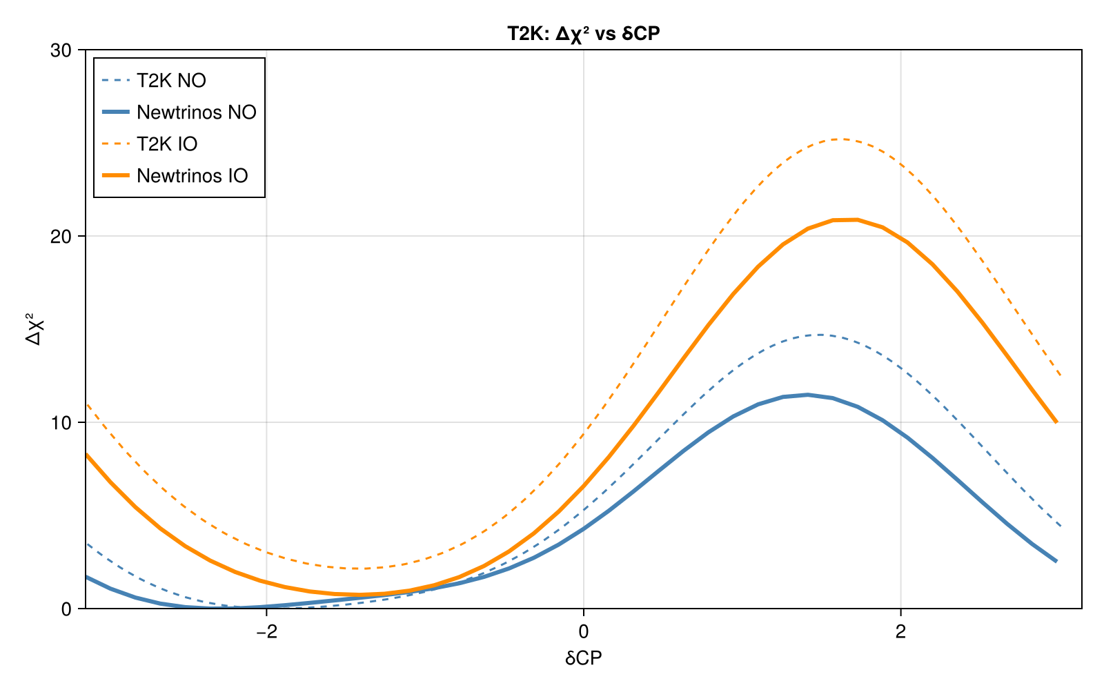
Δχ² as a function of δCP · Fig. 3
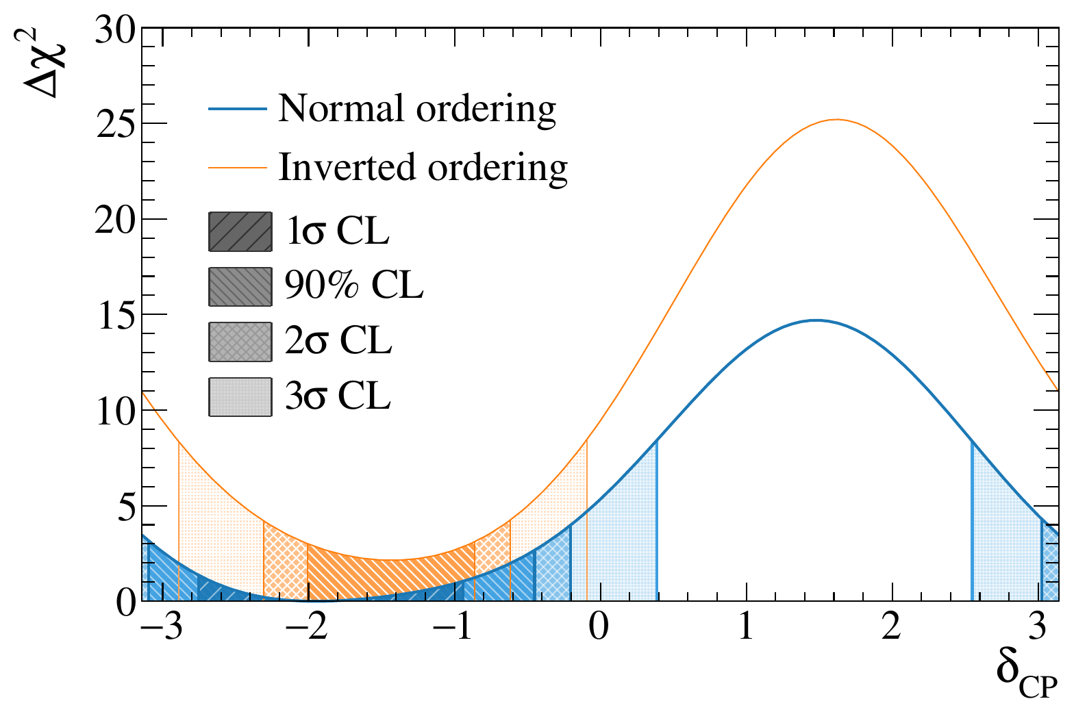
Original figure: T2K, Phys. Rev. Lett. 135, 261801 (2025), Fig. 3, doi:10.1103/gh5j-5cwv. Not our work; shown for comparison, all rights with the authors and publisher.
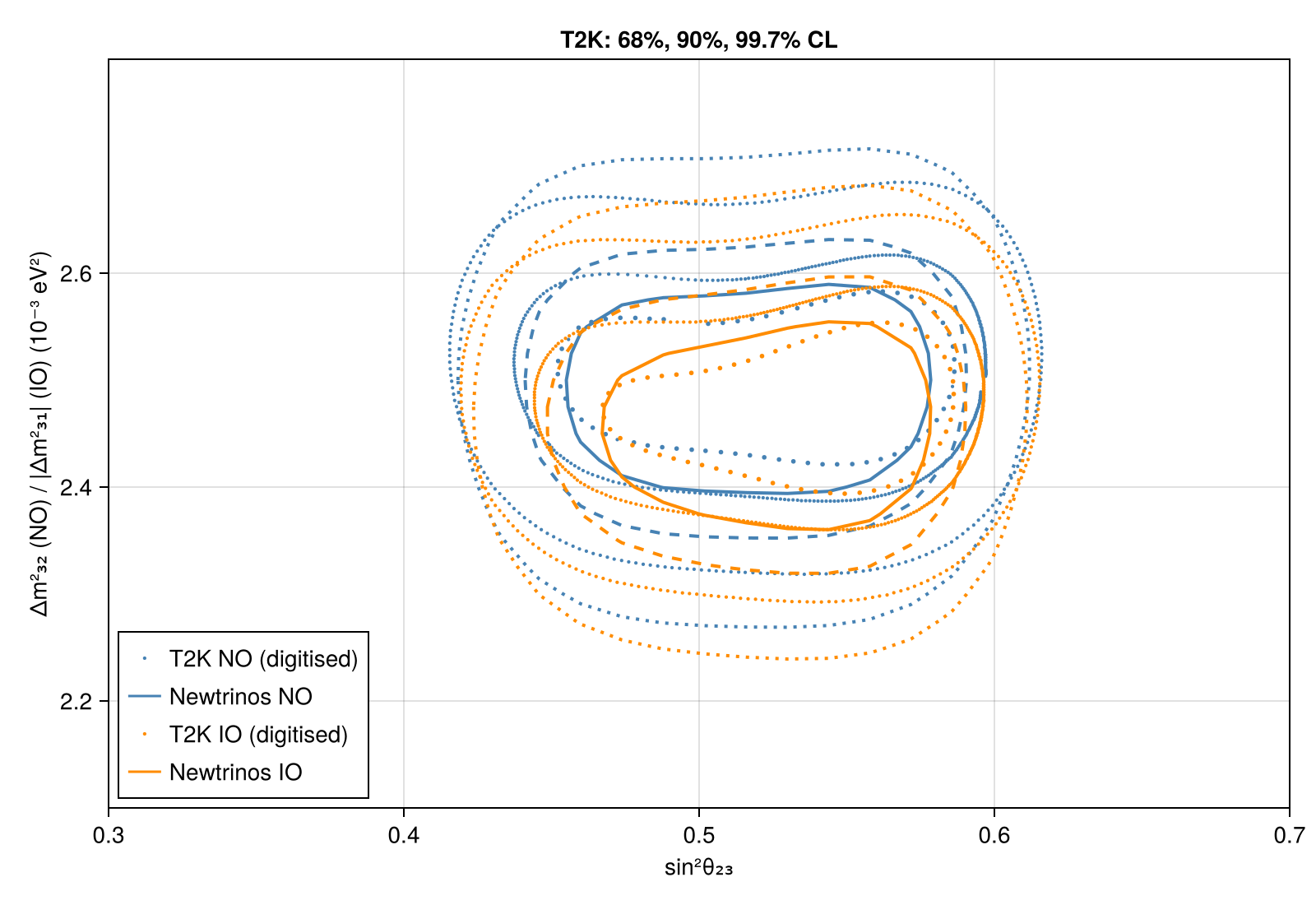
sin²θ₂₃ – Δm², 68%, 90%, 99.7% CL · Fig. 4
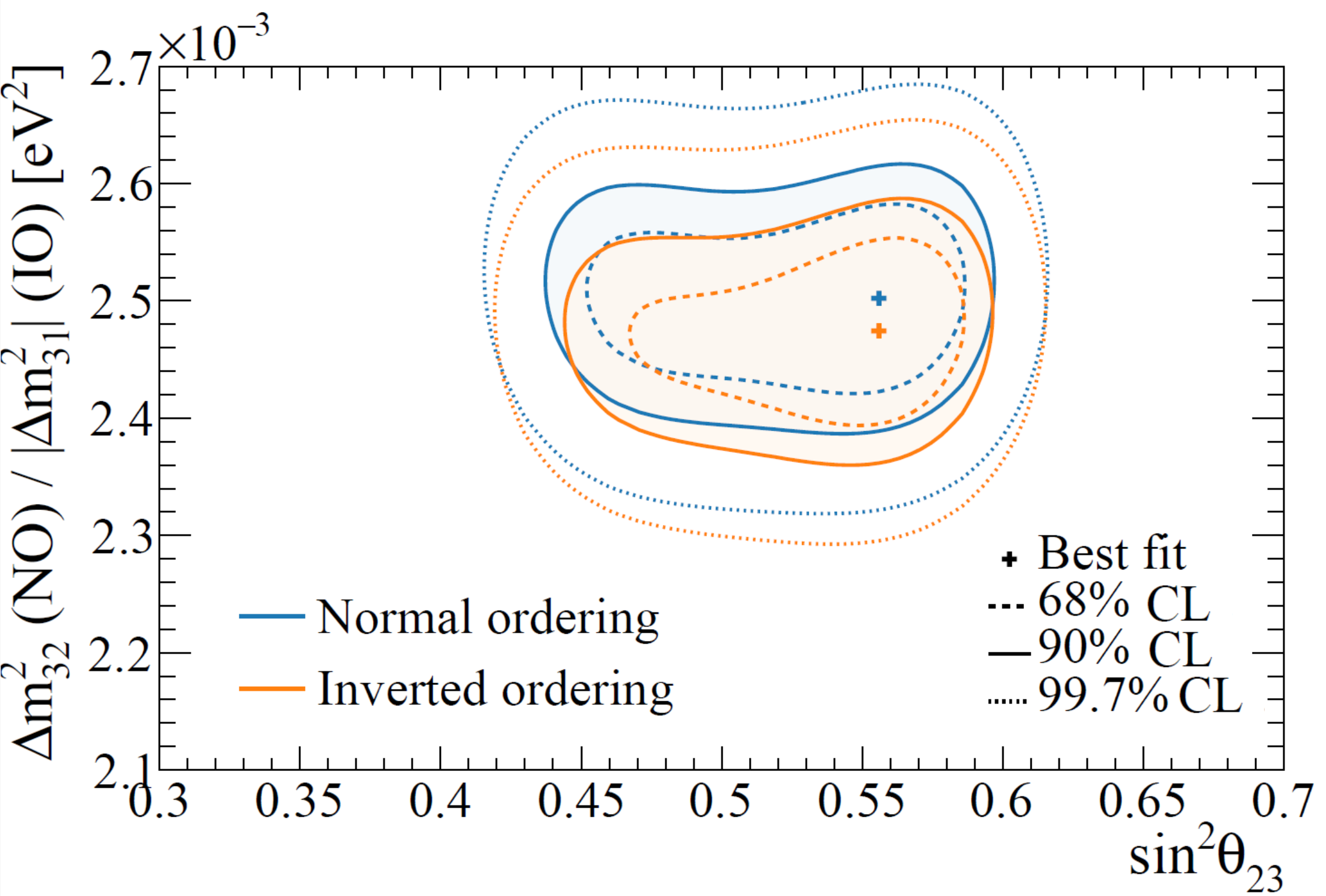
Original figure: T2K, Phys. Rev. Lett. 135, 261801 (2025), Fig. 4, doi:10.1103/gh5j-5cwv. Not our work; shown for comparison, all rights with the authors and publisher.
Known limitations
- The exclusion of δCP ≈ +π/2 and the mass-ordering preference are weaker than official (max Δχ² 11.5 vs 14.7 in NO, IO penalty 0.74 vs ≈ 2.2); the gap remains without any systematics (13.3 in NO), so it is in the predictions or the use of the data (e-like samples are fitted in E_rec only; T2K fits momentum–angle). Spectra and rates: see the T2K 2023 entry.
- Pinned to Newtrinos.jl feature/t2k-numu-bkg (3c346d7): misidentified νμ CC events in the e-like samples now oscillate with P_μμ (before, as beam νe: max Δχ² 10.5 in NO).
- The released predictions are ~5–9% above T2K's own fitted rates; FHC 1Rμ data are 15% below the release prediction.
- The official θ₂₃–Δm² contours are digitised from a raster image; the official Δm² contour is smeared for simulated-data studies.
Reproduce
git clone https://github.com/Newtrinos-org/Newtrinos.jl.git && cd Newtrinos.jl && git checkout 3c346d7f31- Download reproduce.jl into an empty directory.
julia -t 8 --project=/path/to/Newtrinos.jl reproduce.jl
# Reproduction of T2K, Phys. Rev. Lett. 135, 261801 (2025) [arXiv:2506.05889] with Newtrinos.jl (module `t2k`).
# Run from this directory with the Newtrinos.jl environment at the pinned commit:
#   julia -t 8 --project=<path to Newtrinos.jl> reproduce.jl
using Newtrinos, Distributions, DataStructures, Accessors, FileIO, CairoMakie, HDF5, CSV, DataFrames

cd(@__DIR__); mkpath("ours"); mkpath("results"); mkpath("cache")

# CSV export of a profile scan: one row per grid point, ASCII column names, oscillation parameters in physical
# units (sin²θ, Δm²₃₂ = Δm²₃₁ − Δm²₂₁ in eV², δCP in rad), dchi2 = -2Δlog L w.r.t. `ref` (default: the scan's best fit)
function save_csv(path, r; ref = maximum(r.values.log_posterior))
    ascii(k) = replace(string(k), "θ" => "theta", "Δm²" => "dm2_", "δ" => "d", "₁" => "1", "₂" => "2", "₃" => "3", "CP" => "cp")
    cols = OrderedDict{String,Any}()
    for (k, v) in pairs(r.values)
        x = vec(v)
        if startswith(string(k), "θ")
            cols["sin2_" * ascii(k)] = sin.(x) .^ 2
        elseif k == :Δm²₃₁
            cols["dm2_32"] = x .- vec(r.values.Δm²₂₁)
        end
        cols[ascii(k)] = x
    end
    cols["dchi2"] = 2 .* (ref .- vec(r.values.log_posterior))
    haskey(cols, "llh") && (cols["log_likelihood"] = pop!(cols, "llh"))
    first_cols = filter(in(keys(cols)), ["sin2_theta23", "dm2_32", "dcp", "dchi2", "log_likelihood", "log_posterior"])
    CSV.write(path, DataFrame(cols)[:, vcat(first_cols, setdiff(collect(keys(cols)), first_cols))])
end

# draw each confidence level with its own line style (1σ solid, 2σ dashed, 3σ dotted)
function contours!(ax, res, levels; color, label)
    for (lv, ls) in zip(levels, (:solid, :dash, :dot))
        plot!(ax, res, levels = [lv], color = color, linestyle = ls, label = lv == first(levels) ? label : nothing)
    end
end

experiments = (t2k = Newtrinos.t2k.configure(),)
likelihood = Newtrinos.generate_likelihood(experiments)
p = Newtrinos.get_params(experiments)
priors = Newtrinos.get_priors(experiments)

# as in the paper: solar parameters fixed, reactor constraint sin²θ₁₃ = 0.0220 ± 0.0007, flat δCP
ref = Newtrinos.t2k.ref_params()
p = merge(p, (θ₁₂ = ref.θ₁₂, Δm²₂₁ = ref.Δm²₂₁, θ₁₃ = ref.θ₁₃))
θ₂₃_range = (asin(sqrt(0.35)), asin(sqrt(0.68)))
priors = merge(priors, (θ₁₂ = p.θ₁₂, Δm²₂₁ = p.Δm²₂₁, θ₁₃ = Normal(ref.θ₁₃, 0.0007 / (2 * sin(ref.θ₁₃) * cos(ref.θ₁₃))),
                        δCP = Uniform(0, 2π), θ₂₃ = Uniform(θ₂₃_range...)))

orderings = (NO = (Δm²₃₁ = (2.2e-3, 2.8e-3) .+ p.Δm²₂₁, start = (Δm²₃₁ = 2.506e-3 + p.Δm²₂₁, δCP = mod(-2.18, 2π)),
                   dm2 = x -> x - p.Δm²₂₁, color = :steelblue),
             IO = (Δm²₃₁ = (-2.8e-3, -2.2e-3), start = (Δm²₃₁ = -2.47e-3, δCP = mod(-1.37, 2π)),
                   dm2 = x -> -x, color = :darkorange))

# the θ₂₃ octants are separate local minima: profile each octant, keep the better one per point
# δCP has several local optima (and optima just across the 0/2π boundary of its prior): each point is fitted from the
# default start and four δCP starts (starts that only set a scanned parameter are dropped)
const STARTS = [(;), ((δCP = k * π / 4,) for k in (1, 3, 5, 7))...]

function profile_octants(pr, p0, vars, cache_dir)
    oct = map((lower = (θ₂₃_range[1], π / 4), upper = (π / 4, θ₂₃_range[2]))) do r
        Newtrinos.profile(likelihood, @set(pr.θ₂₃ = Uniform(r...)), vars, @set(p0.θ₂₃ = sum(r) / 2), cache_dir = cache_dir, starts = STARTS)
    end
    # the two octant scans use θ₂₃ priors of different widths, which shifts each log_posterior by its own
    # constant −log(width): remove it before comparing the octants (nuisance-parameter priors are kept)
    widths = (lower = π / 4 - θ₂₃_range[1], upper = θ₂₃_range[2] - π / 4)
    oct = map((r, w) -> Newtrinos.NewtrinosResult(axes = r.axes, meta = r.meta,
                                                   values = merge(r.values, (log_posterior = r.values.log_posterior .+ log(w),))), oct, widths)
    better = oct.lower.values.log_posterior .>= oct.upper.values.log_posterior
    Newtrinos.NewtrinosResult(axes = oct.lower.axes, values = map((l, u) -> ifelse.(better, l, u), oct.lower.values, oct.upper.values), meta = oct.lower.meta)
end

results = map(keys(orderings), values(orderings)) do mo, o
    pr = @set priors.Δm²₃₁ = Uniform(o.Δm²₃₁...)
    p0 = merge(p, (Δm²₃₁ = o.start.Δm²₃₁, δCP = o.start.δCP, θ₂₃ = asin(sqrt(0.56))))
    th23dm = Newtrinos.profile(likelihood, pr, OrderedDict(:θ₂₃ => 25, :Δm²₃₁ => 25), p0, cache_dir = "cache/$(mo)_th23dm31", starts = STARTS)
    dcp = profile_octants(pr, p0, OrderedDict(:δCP => 41), "cache/$(mo)_dcp")
    FileIO.save("results/t2k_$(mo).jld2", Dict("th23dm31" => th23dm, "dcp" => dcp))
    mo => (; th23dm, dcp)
end |> NamedTuple
# Δχ² references: each scan type carries the log density of its own scanned-parameter priors, so a scan is
# referenced to the best fit over both orderings of the same scan type
scan_max(k) = maximum(r -> maximum(r[k].values.log_posterior), results)
global_max = maximum(r -> maximum(r.dcp.values.log_posterior), results)
for mo in keys(results)   # dchi2 relative to the global best fit over both orderings
    save_csv("results/t2k_$(mo)_ssth23_dm2.csv", results[mo].th23dm; ref = scan_max(:th23dm))
    save_csv("results/t2k_$(mo)_dcp.csv", results[mo].dcp; ref = global_max)
end

official = h5open(Newtrinos.t2k.datafile) do f
    (dcp = Dict(mo => (read(f["official/dcp/$mo/dcp"]), read(f["official/dcp/$mo/dchi2"])) for mo in ("NO", "IO")),
     th23dm2 = Dict(mo => Dict(l => (read(f["official/th23dm2/$mo/$l/ssth23"]), read(f["official/th23dm2/$mo/$l/dm2"])) for l in ("068", "090", "997")) for mo in ("NO", "IO")))
end

# Fig. 3: Δχ²(δCP) relative to the global best fit
wrap(x) = mod(x + π, 2π) - π
fig = Figure(size = (800, 500))
ax = Axis(fig[1, 1], title = "T2K: Δχ² vs δCP", xlabel = "δCP", ylabel = "Δχ²")
for mo in keys(orderings)
    x, y = official.dcp[string(mo)]
    lines!(ax, x, y, color = orderings[mo].color, linestyle = :dash, label = "T2K $(mo)")
    r = results[mo].dcp; d = wrap.(r.axes.δCP); i = sortperm(d)
    lines!(ax, d[i], (2 .* (global_max .- r.values.log_posterior))[i], color = orderings[mo].color, linewidth = 3, label = "Newtrinos $(mo)")
end
xlims!(ax, -π, π); ylims!(ax, 0, 30)
axislegend(ax, position = :lt)
save("ours/fig3_dcp.png", fig)

# Fig. 4: sin²θ₂₃ – Δm²₃₂ (NO) / |Δm²₃₁| (IO), 68%, 90%, 99.7% CL, conditional on each ordering
fig = Figure(size = (800, 550))
ax = Axis(fig[1, 1], title = "T2K: 68%, 90%, 99.7% CL", xlabel = "sin²θ₂₃", ylabel = "Δm²₃₂ (NO) / |Δm²₃₁| (IO) (10⁻³ eV²)")
for mo in keys(orderings)
    o = orderings[mo]
    for (l, ms) in (("068", 4), ("090", 3), ("997", 3))
        x, y = official.th23dm2[string(mo)][l]
        keep = (y .> 2.25e-3) .& (x .< 0.65)          # drop stray digitisation points (legend, labels)
        x, y = x[keep], y[keep]
        scatter!(ax, x, y .* 1e3, color = o.color, markersize = ms, label = l == "090" ? "T2K $(mo) (digitised)" : nothing)
    end
    r = results[mo].th23dm
    contours!(ax, Newtrinos.NewtrinosResult(axes = (ss23 = sin.(r.axes.θ₂₃) .^ 2, dm2 = o.dm2.(r.axes.Δm²₃₁) .* 1e3), values = r.values),
              [0.68, 0.9, 0.997]; color = o.color, label = "Newtrinos $(mo)")
end
xlims!(ax, 0.3, 0.7); ylims!(ax, 2.1, 2.8)
axislegend(ax, position = :lb)
save("ours/fig4_ssth23_dm2.png", fig)
Provenance
| Newtrinos.jl commit | 3c346d7f31 (t2k) |
|---|---|
| Run date | 2026-10-15T11:06:11Z |
| Wall time | 5.3 min (32 threads) |
| Julia | 1.12.5 |
| Machine | AMD EPYC 7702P 64-Core Processor, 128 hardware threads, Linux |
| Environment | newtrinos_Manifest.toml · run.toml |
Downloads
CSV files hold one row per scan point: the scanned and profiled parameters
(sin2_theta23, dm2_32 in eV², dcp in rad, nuisance parameters), dchi2 = −2Δ log L
and the log-likelihood. JLD2 files contain the full NewtrinosResult objects.
| File | Size | SHA-256 |
|---|---|---|
| ours/fig3_dcp.png | 114.5 kB | 5bf166130e14… |
| ours/fig4_ssth23_dm2.png | 223.7 kB | 253e88cc07c8… |
| results/t2k_IO.jld2 | 154.2 kB | 154ef3400880… |
| results/t2k_IO_dcp.csv | 19.9 kB | 516ca3c86208… |
| results/t2k_IO_ssth23_dm2.csv | 284.9 kB | bf3a273d453a… |
| results/t2k_NO.jld2 | 154.2 kB | 3e739187b904… |
| results/t2k_NO_dcp.csv | 19.9 kB | bc5d23654fae… |
| results/t2k_NO_ssth23_dm2.csv | 283.9 kB | 80d9015fae61… |