
T2K · Eur. Phys. J. C 83, 782 (2023)
Measurements of neutrino oscillation parameters from the T2K experiment using 3.6×10²¹ protons on target
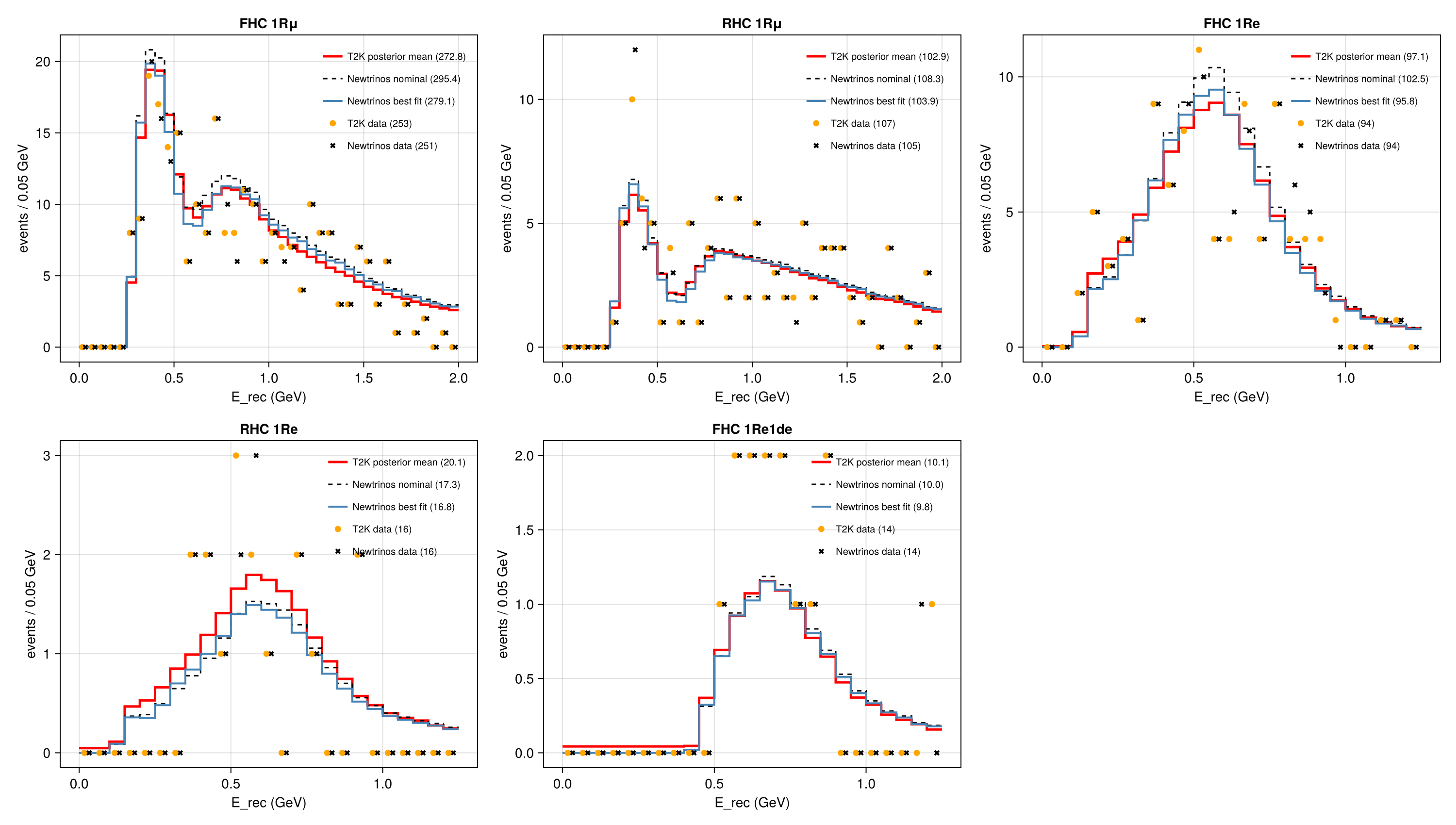
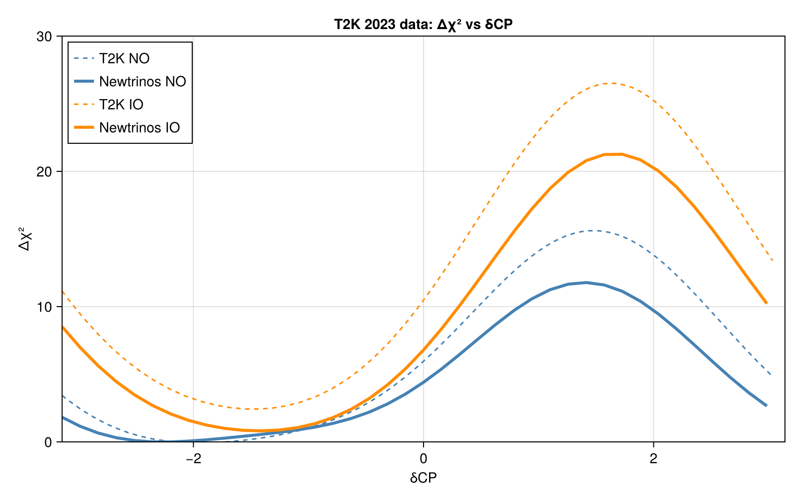
The Newtrinos t2k module uses the far-detector data events of this paper and the predictions of the 2025 T2K data release (same exposure, 19.7 (16.3)×10²⁰ POT in ν (ν̄) mode, newer near-detector fit). Compared here: the binned E_rec data and T2K's mean posterior prediction (Fig. 27), the predicted event rates vs δCP (Tab. 9) and Δχ²(δCP) from the data with the reactor constraint (Fig. 28). Inputs extracted from the vector figures of the arXiv source (data/extract.py).
Figures
Far-detector E_rec spectra: data and predictions · Fig. 27
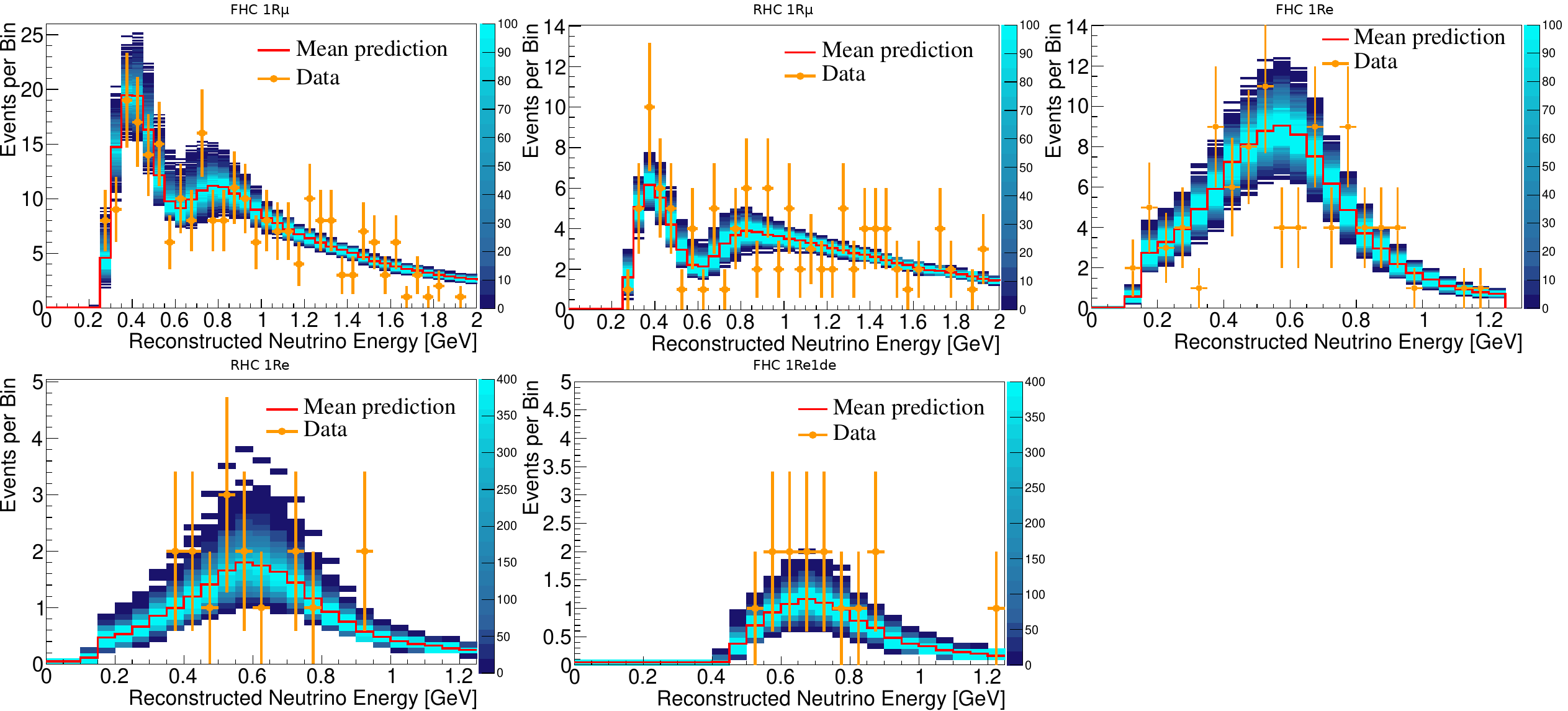
Original figure: T2K, Eur. Phys. J. C 83, 782 (2023), Fig. 27, doi:10.1140/epjc/s10052-023-11819-x. Not our work; shown for comparison, all rights with the authors and publisher.
Δχ² as a function of δCP (reactor constraint) · Fig. 28
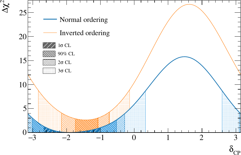
Original figure: T2K, Eur. Phys. J. C 83, 782 (2023), Fig. 28, doi:10.1140/epjc/s10052-023-11819-x. Not our work; shown for comparison, all rights with the authors and publisher.
Known limitations
- The binned data agree: e-like 94 / 16 / 14 events in both, μ-like within ±2 events per sample below 2 GeV; single bins differ by ±1 event (E_rec reconstruction at bin edges).
- T2K's mean posterior prediction (Bayesian, without reactor constraint) lies 5–8% below the release nominal in the FHC samples (1Rμ −7.7% below 2 GeV, about uniform in energy), i.e. T2K's fit lands below the nominal we start from; part of this may be the change of near-detector fit between the 2023 analysis and the 2025 release.
- Our δCP best fits are close (NO −2.2 in a flat valley from −2.6 to −1.5, official −1.97; IO −1.41, official −1.44; Δχ²(+π/2) 11.6 / 21.2, official 15.6 / 26.5); the exclusion of δCP ≈ +π/2 and the IO penalty are weaker than official: our fit absorbs the data deficit partly by θ₂₃ → maximal mixing, which lowers the e-like rate at δCP = −π/2.
- e-like samples are fitted in E_rec only (T2K fits momentum–angle); the paper attributes the stronger-than-expected δCP constraint to the FHC 1Re1de sample (14 events observed, ~10 expected).
- Pinned to Newtrinos.jl feature/t2k-numu-bkg (3c346d7): misidentified νμ CC events in the e-like samples oscillate with P_μμ (before, treated as beam νe: NO Δχ²(+π/2) 10.5).
Reproduce
git clone https://github.com/Newtrinos-org/Newtrinos.jl.git && cd Newtrinos.jl && git checkout 3c346d7f31- Download reproduce.jl and the
data/folder of this entry into an empty directory. julia -t 8 --project=/path/to/Newtrinos.jl reproduce.jl
# Comparison with T2K, Eur. Phys. J. C 83, 782 (2023) [arXiv:2303.03222] with Newtrinos.jl (module `t2k`):
# the far-detector E_rec spectra (data and mean posterior prediction, Fig. 27), the predicted e-like event rates vs δCP
# (Tab. 9) and Δχ²(δCP) from the data (Fig. 28). The `t2k` module uses the data events of this paper and the
# predictions of the 2025 data release (same exposure, newer near-detector fit).
# Run from this directory with the Newtrinos.jl environment at the pinned commit:
#   julia -t 8 --project=<path to Newtrinos.jl> reproduce.jl
using Newtrinos, Distributions, DataStructures, Accessors, FileIO, CairoMakie, CSV, DataFrames, Printf

cd(@__DIR__); mkpath("ours"); mkpath("results"); mkpath("cache")
const T = Newtrinos.t2k

experiments = (t2k = T.configure(),)
e = experiments.t2k
likelihood = Newtrinos.generate_likelihood(experiments)
p = Newtrinos.get_params(experiments)
priors = Newtrinos.get_priors(experiments)

# as in the paper: solar parameters fixed, reactor constraint sin²2θ₁₃ = 0.0853 ± 0.0027 (sin²θ₁₃ = 0.0218 ± 0.0007),
# flat δCP and sin²θ₂₃
ref = T.ref_params()
θ13 = asin(sqrt(0.0218))
p = merge(p, (θ₁₂ = ref.θ₁₂, Δm²₂₁ = ref.Δm²₂₁, θ₁₃ = θ13))
θ₂₃_range = (asin(sqrt(0.35)), asin(sqrt(0.68)))
priors = merge(priors, (θ₁₂ = p.θ₁₂, Δm²₂₁ = p.Δm²₂₁, θ₁₃ = Normal(θ13, 0.0007 / sin(2θ13)), δCP = Uniform(0, 2π),
                        θ₂₃ = Uniform(θ₂₃_range...)))

orderings = (NO = (Δm²₃₁ = (2.2e-3, 2.8e-3) .+ p.Δm²₂₁, start = (Δm²₃₁ = 2.494e-3 + p.Δm²₂₁, δCP = mod(-1.97, 2π)), color = :steelblue),
             IO = (Δm²₃₁ = (-2.8e-3, -2.2e-3), start = (Δm²₃₁ = -2.463e-3, δCP = mod(-1.44, 2π)), color = :darkorange))

# the θ₂₃ octants are separate local minima: profile each octant, keep the better one per point; each point is
# fitted from the default start and four δCP starts
const STARTS = [(;), ((δCP = k * π / 4,) for k in (1, 3, 5, 7))...]
function profile_octants(pr, p0, vars, cache_dir)
    oct = map((lower = (θ₂₃_range[1], π / 4), upper = (π / 4, θ₂₃_range[2]))) do r
        Newtrinos.profile(likelihood, @set(pr.θ₂₃ = Uniform(r...)), vars, @set(p0.θ₂₃ = sum(r) / 2), cache_dir = cache_dir, starts = STARTS)
    end
    # remove the octant-dependent constant −log(width) of the flat θ₂₃ prior before comparing the octants
    widths = (lower = π / 4 - θ₂₃_range[1], upper = θ₂₃_range[2] - π / 4)
    oct = map((r, w) -> Newtrinos.NewtrinosResult(axes = r.axes, meta = r.meta,
                                                   values = merge(r.values, (log_posterior = r.values.log_posterior .+ log(w),))), oct, widths)
    better = oct.lower.values.log_posterior .>= oct.upper.values.log_posterior
    Newtrinos.NewtrinosResult(axes = oct.lower.axes, values = map((l, u) -> ifelse.(better, l, u), oct.lower.values, oct.upper.values), meta = oct.lower.meta)
end

dcp = map(keys(orderings), values(orderings)) do mo, o
    pr = @set priors.Δm²₃₁ = Uniform(o.Δm²₃₁...)
    p0 = merge(p, (Δm²₃₁ = o.start.Δm²₃₁, δCP = o.start.δCP))
    mo => profile_octants(pr, p0, OrderedDict(:δCP => 41), "cache/$(mo)_dcp")
end |> NamedTuple
global_max = maximum(r -> maximum(r.values.log_posterior), dcp)
wrap(x) = mod(x + π, 2π) - π
rows = DataFrame(ordering = String[], dcp = Float64[], dchi2 = Float64[], sin2_theta23 = Float64[], dm2_31 = Float64[])
for mo in keys(dcp), i in eachindex(dcp[mo].axes.δCP)
    v = dcp[mo].values
    push!(rows, (string(mo), wrap(dcp[mo].axes.δCP[i]), 2 * (global_max - v.log_posterior[i]), sin(v.θ₂₃[i])^2, v.Δm²₃₁[i]))
end
sort!(rows, [:ordering, :dcp]); CSV.write("results/dcp.csv", rows)

# best fit (NO or IO) of the δCP scan: all parameters, for the spectra
best = let (mo, i) = argmax(((mo, i),) -> dcp[mo].values.log_posterior[i], [(mo, i) for mo in keys(dcp) for i in eachindex(dcp[mo].axes.δCP)])
    v = dcp[mo].values
    NamedTuple{keys(p)}(Tuple(v[k][i] for k in keys(p)))
end
CSV.write("results/bestfit.csv", DataFrame([string(k) => [best[k]] for k in keys(best)]))

# Fig. 28: Δχ²(δCP) relative to the global best fit
official = CSV.read("data/fig28_dcp.csv", DataFrame)
fig = Figure(size = (800, 500))
ax = Axis(fig[1, 1], title = "T2K 2023 data: Δχ² vs δCP", xlabel = "δCP", ylabel = "Δχ²")
for mo in keys(orderings)
    off = official[official.ordering .== string(mo), :]
    lines!(ax, off.dcp, off.dchi2, color = orderings[mo].color, linestyle = :dash, label = "T2K $(mo)")
    r = rows[rows.ordering .== string(mo), :]
    lines!(ax, r.dcp, r.dchi2, color = orderings[mo].color, linewidth = 3, label = "Newtrinos $(mo)")
end
xlims!(ax, -π, π); ylims!(ax, 0, 30)
axislegend(ax, position = :lt)
save("ours/fig28_dcp.png", fig)

# Tab. 9: predicted e-like events vs δCP at the release reference point (nominal systematics); official: at T2K's
# best-fit oscillation and systematic parameters
tab9 = (fhc1rmu = [346.61, 345.90, 346.57, 347.38], rhc1rmu = [135.80, 135.45, 135.81, 136.19],
        fhc1re = [96.55, 81.59, 66.89, 81.85], rhc1re = [16.56, 18.81, 20.75, 18.49], fhc1re1de = [9.30, 8.10, 6.59, 7.79])
dvals = (-π / 2, 0.0, π / 2, π)
rates = DataFrame(sample = String[], dcp = Float64[], newtrinos = Float64[], t2k = Float64[], observed = Int[])
for k in keys(tab9), (j, d) in enumerate(dvals)
    λ = T.get_expected(merge(p, ref, (δCP = mod(d, 2π),)), e.physics, e.assets)[k]
    push!(rates, (string(k), d, sum(λ), tab9[k][j], sum(e.assets.observed[k])))
end
CSV.write("results/tab9_rates.csv", rates)

# Fig. 27: E_rec spectra. T2K: data and mean posterior prediction (Bayesian, without reactor constraint);
# Newtrinos: data, nominal prediction at the release reference point and at our best fit
pp = CSV.read("data/fig27_postpred.csv", DataFrame)
samples = (FHC1Rmu = (:fhc1rmu, "FHC 1Rμ"), RHC1Rmu = (:rhc1rmu, "RHC 1Rμ"), FHC1Re = (:fhc1re, "FHC 1Re"),
           RHC1Re = (:rhc1re, "RHC 1Re"), FHC1Re1de = (:fhc1re1de, "FHC 1Re1de"))
nominal = T.get_expected(merge(p, ref), e.physics, e.assets)
bestexp = T.get_expected(best, e.physics, e.assets)
fig = Figure(size = (1500, 850))
spec = DataFrame(sample = String[], erec_lo = Float64[], erec_hi = Float64[], data_t2k = Int[], data_newtrinos = Int[],
                 posterior_mean_t2k = Float64[], nominal_newtrinos = Float64[], bestfit_newtrinos = Float64[])
for (n, (kk, (k, title))) in enumerate(pairs(samples))
    t = pp[pp.sample .== string(kk), :]
    ed = e.assets.samples[k].target
    idx = [findfirst(x -> isapprox(x, lo, atol = 1e-6), ed) for lo in t.erec_lo]
    keep = .!isnothing.(idx); t = t[keep, :]; idx = Int.(idx[keep])
    od = e.assets.observed[k][idx]; nom = nominal[k][idx]; bf = bestexp[k][idx]
    append!(spec, DataFrame(sample = string(kk), erec_lo = t.erec_lo, erec_hi = t.erec_hi, data_t2k = t.data, data_newtrinos = od,
                            posterior_mean_t2k = t.posterior_mean, nominal_newtrinos = nom, bestfit_newtrinos = bf))
    edges = vcat(t.erec_lo, t.erec_hi[end]); x = (t.erec_lo .+ t.erec_hi) ./ 2
    ax = Axis(fig[(n - 1) ÷ 3 + 1, (n - 1) % 3 + 1], title = title, xlabel = "E_rec (GeV)", ylabel = "events / 0.05 GeV")
    st(y; kw...) = stairs!(ax, edges, vcat(y, y[end]); step = :post, kw...)
    st(t.posterior_mean; color = :red, linewidth = 2.5, label = @sprintf("T2K posterior mean (%.1f)", sum(t.posterior_mean)))
    st(nom; color = :black, linewidth = 1.5, linestyle = :dash, label = @sprintf("Newtrinos nominal (%.1f)", sum(nom)))
    st(bf; color = :steelblue, linewidth = 2, label = @sprintf("Newtrinos best fit (%.1f)", sum(bf)))
    scatter!(ax, x .- 0.008, t.data, color = :orange, markersize = 9, label = "T2K data ($(sum(t.data)))")
    scatter!(ax, x .+ 0.008, od, color = :black, marker = :xcross, markersize = 8, label = "Newtrinos data ($(sum(od)))")
    axislegend(ax, position = :rt, labelsize = 10, framevisible = false)
end
CSV.write("results/spectra.csv", spec)
save("ours/fig27_spectra.png", fig)

for mo in keys(dcp)
    r = rows[rows.ordering .== string(mo), :]
    @printf("%s: min Δχ² %.2f at δCP %.2f, Δχ²(+π/2) %.2f\n", mo, minimum(r.dchi2), r.dcp[argmin(r.dchi2)], r.dchi2[argmin(abs.(r.dcp .- π / 2))])
end
Provenance
| Newtrinos.jl commit | 3c346d7f31 (t2k) |
|---|---|
| Run date | 2026-10-15T11:03:15Z |
| Wall time | 2.2 min (32 threads) |
| Julia | 1.12.5 |
| Machine | AMD EPYC 7702P 64-Core Processor, 128 hardware threads, Linux |
| Environment | newtrinos_Manifest.toml · run.toml |
Downloads
CSV files hold one row per scan point: the scanned and profiled parameters
(sin2_theta23, dm2_32 in eV², dcp in rad, nuisance parameters), dchi2 = −2Δ log L
and the log-likelihood. JLD2 files contain the full NewtrinosResult objects.
| File | Size | SHA-256 |
|---|---|---|
| ours/fig27_spectra.png | 382.2 kB | 5c55931e7daf… |
| ours/fig28_dcp.png | 119.8 kB | d2f33a6f5703… |
| results/bestfit.csv | 626 B | d94d88449a6a… |
| results/dcp.csv | 6.5 kB | 76a19e2bdd6f… |
| results/spectra.csv | 9.4 kB | 73dee4001eab… |
| results/tab9_rates.csv | 1.0 kB | f2035924c4f0… |