
M. Bustamante · arXiv:1904.12391 (2019)
NuOscProbExact: a fast, general-purpose code to compute exact two-, three-, and four-flavor neutrino oscillation probabilities
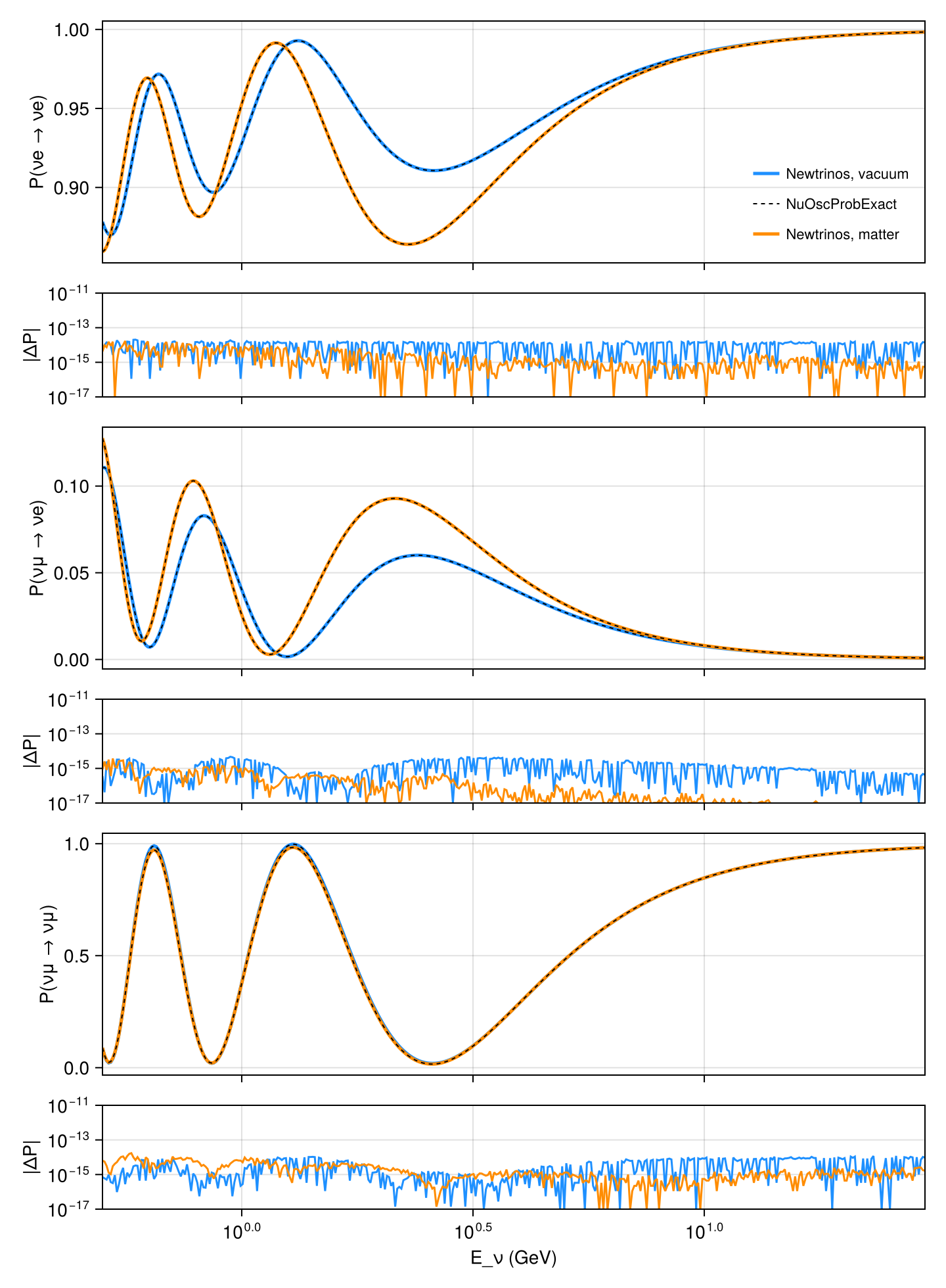
Code benchmark of the Newtrinos.jl oscillation engine (module osc) against NuOscProbExact (version 1.14.0), an exact solver for arbitrary time-independent Hamiltonians: all nine three-flavour channels in vacuum and in matter of constant density for L = 1300 km (the paper's Fig. 2 setting), and ν̄μ survival in a 3+1 model through the Earth (the paper's sterile-neutrino Earth oscillogram), on the default four-zone Newtrinos Earth. The reference values are generated by data/nuoscprobexact_reference.py with the same physical constants as osc.jl and NuOscProbExact's default parameters (NuFit 4.0, normal ordering); for the Earth case the chords through the Newtrinos layers are computed independently and one exact evolution operator per slab is composed.
Figures
Three-flavour probabilities at L = 1300 km, vacuum and matter, and |ΔP| to NuOscProbExact · Fig. 2
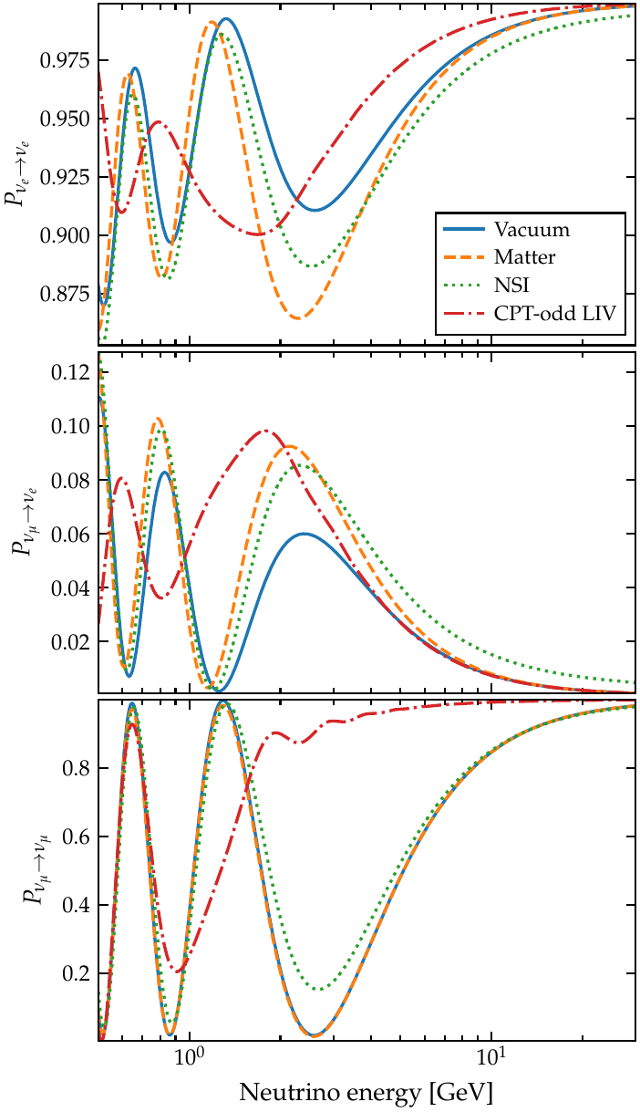
Original figure: M. Bustamante, arXiv:1904.12391 (2019), Fig. 2, doi:10.48550/arXiv.1904.12391. Not our work; shown for comparison, all rights with the authors and publisher.
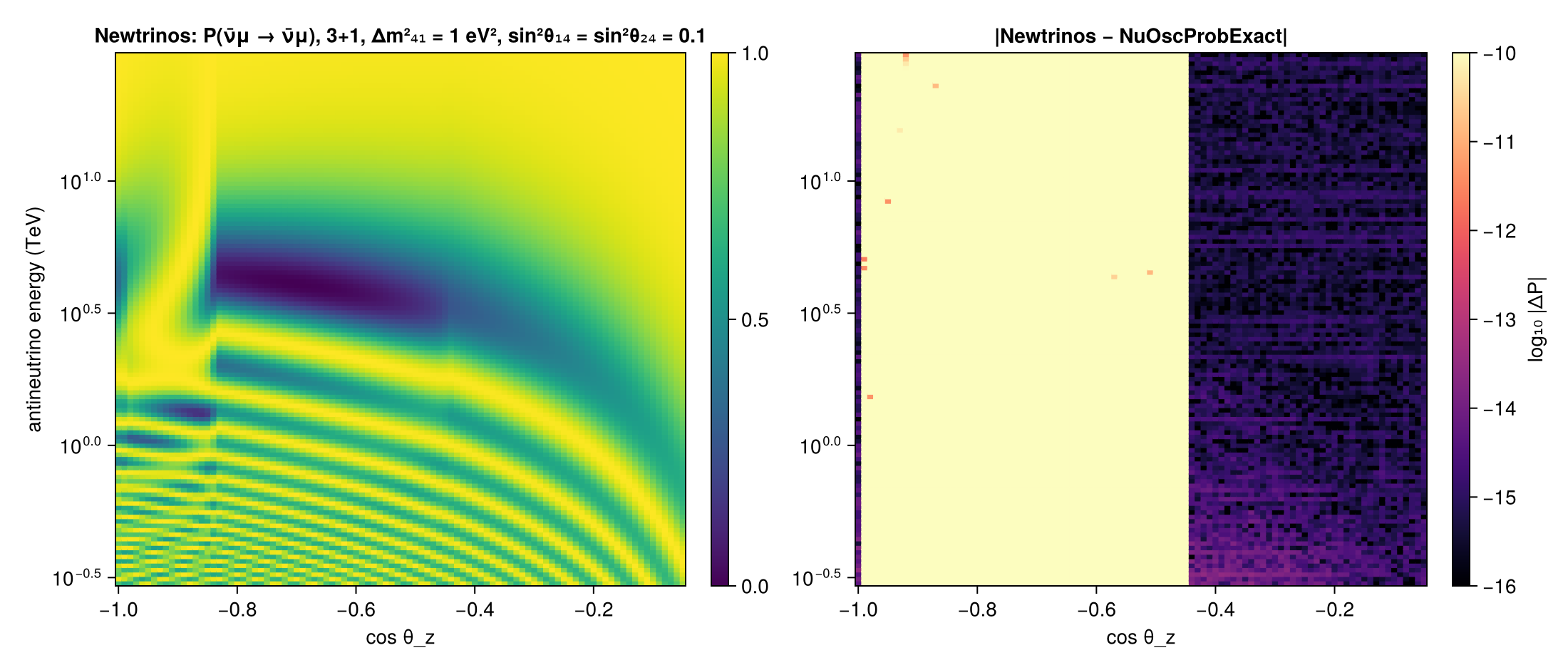
3+1: ν̄μ survival through the Earth, and |ΔP| to NuOscProbExact · sterile-neutrino Earth oscillogram
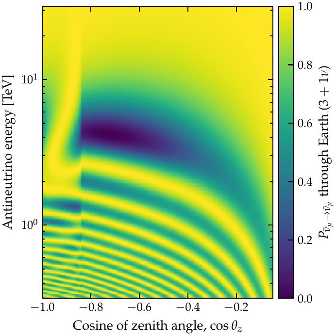
Original figure: M. Bustamante, arXiv:1904.12391 (2019), sterile-neutrino Earth oscillogram, doi:10.48550/arXiv.1904.12391. Not our work; shown for comparison, all rights with the authors and publisher.
Known limitations
- Three flavours, vacuum and constant density: Newtrinos and NuOscProbExact agree to ≤ 2·10⁻¹⁴ in all channels (machine precision).
- 3+1 through the Earth: agreement to ≤ 10⁻¹⁴ for chords that stay in the outer Earth zone (cos θ_z > −0.45) and for cos θ_z = −1; for chords entering deeper zones the probabilities differ by up to 2·10⁻⁵. The cause is the chord geometry in earth_layers.compute_paths: the zone containing the detector (r = 6369 km) is split into its far- and near-side parts with the vertical-path approximation −cos θ_z (R − r_det) instead of the exact chord, e.g. 1266.26 / 1265.06 km instead of 1267.32 / 1263.99 km at cos θ_z = −0.6 (total length exact). Physically negligible.
- The oscillogram is computed on the default four-zone Earth of Newtrinos, not on the finely layered PREM of the paper's figure, so it differs in detail from the original (see the PREM and oscillogram entries for the effect of the layering).
- Non-standard interactions and Lorentz violation (also in the paper's Fig. 2) are not compared here; NSI will be added when it is merged into Newtrinos.
Reproduce
git clone https://github.com/Newtrinos-org/Newtrinos.jl.git && cd Newtrinos.jl && git checkout de27463fde- Download reproduce.jl and the
data/folder of this entry into an empty directory. julia -t 8 --project=/path/to/Newtrinos.jl reproduce.jl
# Newtrinos.jl oscillation probabilities (module `osc`: three flavours in vacuum and matter, 3+1 sterile through the
# Earth) compared with NuOscProbExact (M. Bustamante, arXiv:1904.12391), an exact solver for arbitrary Hamiltonians.
# The NuOscProbExact reference values are produced by data/nuoscprobexact_reference.py (pip install nuoscprobexact).
# Run from this directory with the Newtrinos.jl environment at the pinned commit:
#   julia --project=<path to Newtrinos.jl> reproduce.jl
using Newtrinos, CairoMakie, CSV, DataFrames, Printf, StructArrays, ArraysOfArrays

cd(@__DIR__); mkpath("ours"); mkpath("results")
pj = CSV.read("data/ref_parameters.csv", DataFrame)[1, :]
p3 = (θ₁₂ = asin(pj["s12"]), θ₁₃ = asin(pj["s13"]), θ₂₃ = asin(pj["s23"]), δCP = pj["dcp"], Δm²₂₁ = pj["d21"], Δm²₃₁ = pj["d31"])
p4 = (; p3..., Δm²₄₁ = pj["d41"], θ₁₄ = asin(pj["s14"]), θ₂₄ = asin(pj["s24"]), θ₃₄ = asin(pj["s34"]))

# ---------------- (1) three flavours, L = 1300 km: vacuum and constant density ρ = 3 g/cm³, Yₑ = 0.5 ----------------
ref = CSV.read("data/ref_3nu_1300km.csv", DataFrame)
E = ref.E_GeV
vac = Newtrinos.osc.configure(Newtrinos.osc.OscillationConfig())
mat = Newtrinos.osc.configure(Newtrinos.osc.OscillationConfig(interaction = Newtrinos.osc.SI()))
crust = StructArray{Newtrinos.Layer}(([7000.0], [1.5], [1.5]))
path = VectorOfVectors{Newtrinos.Path}([StructArray{Newtrinos.Path}(([1300.0], [1]))])
P = (vacuum = vac.osc_prob(E, [1300.0], p3)[:, 1, :, :], matter = mat.osc_prob(E, path, crust, p3)[:, 1, :, :])
CH = [("Pee", 1, 1), ("Pem", 1, 2), ("Pet", 1, 3), ("Pme", 2, 1), ("Pmm", 2, 2), ("Pmt", 2, 3), ("Pte", 3, 1), ("Ptm", 3, 2), ("Ptt", 3, 3)]
rows = [(case = String(c), channel = n, max_abs_diff = maximum(abs.(P[c][:, a, b] .- ref[!, "$(c)_$n"]))) for c in (:vacuum, :matter) for (n, a, b) in CH]

fig = Figure(size = (720, 980))
for (k, (n, a, b, lab)) in enumerate((("Pee", 1, 1, "P(νe → νe)"), ("Pme", 2, 1, "P(νμ → νe)"), ("Pmm", 2, 2, "P(νμ → νμ)")))
    ax = Axis(fig[2k - 1, 1], xscale = log10, ylabel = lab, xticklabelsvisible = false, limits = (0.5, 30, nothing, nothing))
    for (c, col, lb) in ((:vacuum, :dodgerblue, "vacuum"), (:matter, :darkorange, "matter"))
        lines!(ax, E, P[c][:, a, b], color = col, linewidth = 2.5, label = "Newtrinos, $lb")
        lines!(ax, E, ref[!, "$(c)_$n"], color = :black, linestyle = :dash, linewidth = 1, label = c == :vacuum ? "NuOscProbExact" : nothing)
    end
    k == 1 && axislegend(ax, position = :rb, framevisible = false, labelsize = 11)
    axd = Axis(fig[2k, 1], xscale = log10, yscale = log10, ylabel = "|ΔP|", limits = (0.5, 30, 1e-17, 1e-11),
               xlabel = k == 3 ? "E_ν (GeV)" : "", xticklabelsvisible = k == 3, yticks = LogTicks(-17:2:-11))
    for (c, col) in ((:vacuum, :dodgerblue), (:matter, :darkorange))
        lines!(axd, E, max.(abs.(P[c][:, a, b] .- ref[!, "$(c)_$n"]), 1e-17), color = col)
    end
    rowsize!(fig.layout, 2k, Relative(0.1))
end
save("ours/fig_prob_3nu_vs_energy.png", fig)

# ---------------- (2) 3+1: ν̄μ survival through the Earth (default four-zone Newtrinos Earth) ----------------
ref4 = CSV.read("data/ref_3p1_earth_numubar.csv", DataFrame)
CZ, E4 = unique(ref4.cz), unique(ref4.E_GeV)
Pref = permutedims(reshape(ref4.Pmm_bar, length(E4), length(CZ)))          # [cz, E]
earth = Newtrinos.earth_layers.configure()
layers = earth.compute_layers()
ster = Newtrinos.osc.configure(Newtrinos.osc.OscillationConfig(flavour = Newtrinos.osc.Sterile(), interaction = Newtrinos.osc.SI()))
Pn = permutedims(ster.osc_prob(E4, earth.compute_paths(CZ, layers), layers, p4; anti = true)[:, :, 2, 2])   # [cz, E]
push!(rows, (case = "3+1 Earth", channel = "P(ν̄μ → ν̄μ)", max_abs_diff = maximum(abs.(Pn .- Pref))))

fig = Figure(size = (1100, 470))
ax = Axis(fig[1, 1], yscale = log10, xlabel = "cos θ_z", ylabel = "antineutrino energy (TeV)",
          title = "Newtrinos: P(ν̄μ → ν̄μ), 3+1, Δm²₄₁ = 1 eV², sin²θ₁₄ = sin²θ₂₄ = 0.1")
hm = heatmap!(ax, CZ, E4 ./ 1e3, Pn, colormap = :viridis, colorrange = (0, 1))
Colorbar(fig[1, 2], hm)
ax2 = Axis(fig[1, 3], yscale = log10, xlabel = "cos θ_z", title = "|Newtrinos − NuOscProbExact|")
hm2 = heatmap!(ax2, CZ, E4 ./ 1e3, log10.(max.(abs.(Pn .- Pref), 1e-17)), colormap = :magma, colorrange = (-16, -10))
Colorbar(fig[1, 4], hm2, label = "log₁₀ |ΔP|")
save("ours/fig_sterile_earth.png", fig)

tab = DataFrame(rows)
CSV.write("results/max_abs_differences.csv", tab)
show(stdout, tab, allrows = true); println()
Provenance
| Newtrinos.jl commit | de27463fde (osc (ThreeFlavour, Sterile; Vacuum, SI), earth_layers) |
|---|---|
| Run date | 2026-10-05T08:14:41Z |
| Wall time | 1.4 min (2 threads) |
| Julia | 1.13.0 |
| Machine | 13th Gen Intel(R) Core(TM) i7-13700H, 20 hardware threads, Linux |
| Environment | newtrinos_Manifest.toml · run.toml |
Downloads
CSV files hold one row per scan point: the scanned and profiled parameters
(sin2_theta23, dm2_32 in eV², dcp in rad, nuisance parameters), dchi2 = −2Δ log L
and the log-likelihood. JLD2 files contain the full NewtrinosResult objects.
| File | Size | SHA-256 |
|---|---|---|
| ours/fig_prob_3nu_vs_energy.png | 455.8 kB | 4395c5d700aa… |
| ours/fig_sterile_earth.png | 285.6 kB | 61055bcf2c9f… |
| results/max_abs_differences.csv | 676 B | d9766ac7aaea… |