
Y. Herrera, A. Serenelli · Zenodo, v1.2 (2023)
Standard Solar Models B23 / SF-III
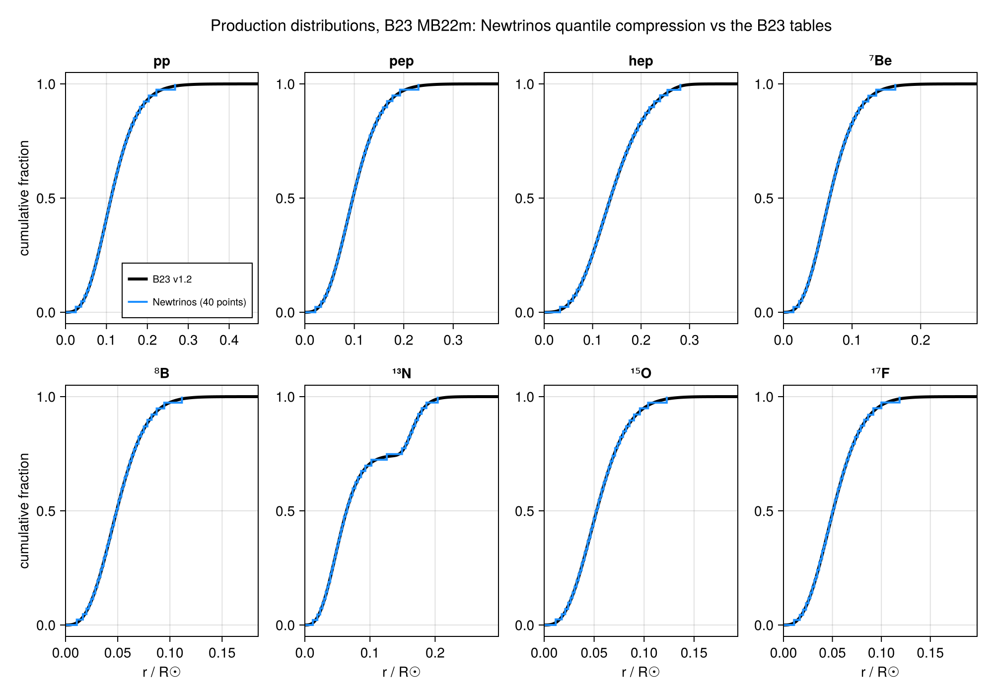
The B23 standard solar models (Herrera & Serenelli, SF-III nuclear rates; MB22-met is the NuFIT 6.0 reference) as used by Newtrinos' solar_flux module, compared with the B23 package (v1.2) and with the B23 fluxes published in Solar fusion III (Rev. Mod. Phys. 97, 035002 (2025), Table II). The fluxes agree with Table II within its rounding for GS98, AAG21 and MB22p, and are identical to the package for all six compositions; the correlated flux prior (solar_norms) reproduces the package's uncertainties and correlation matrices to 10⁻¹⁶. The electron density used for the MSW conversion agrees with B23 to 5×10⁻⁷ from the centre to the surface, and the 40-point production regions reproduce the B23 production distributions (mean radius and mean nₑ at production identical to 10⁻⁴).
Figures
B23 fluxes and uncertainties: Newtrinos vs Solar fusion III, Table II (GS98, AAG21, MB22p) · Solar fusion III, Table II
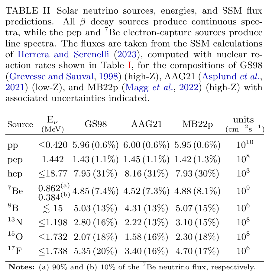
Original figure: Y. Herrera, A. Serenelli, Zenodo, v1.2 (2023), Solar fusion III, Table II, doi:10.5281/zenodo.10174170. Not our work; shown for comparison, all rights with the authors and publisher.
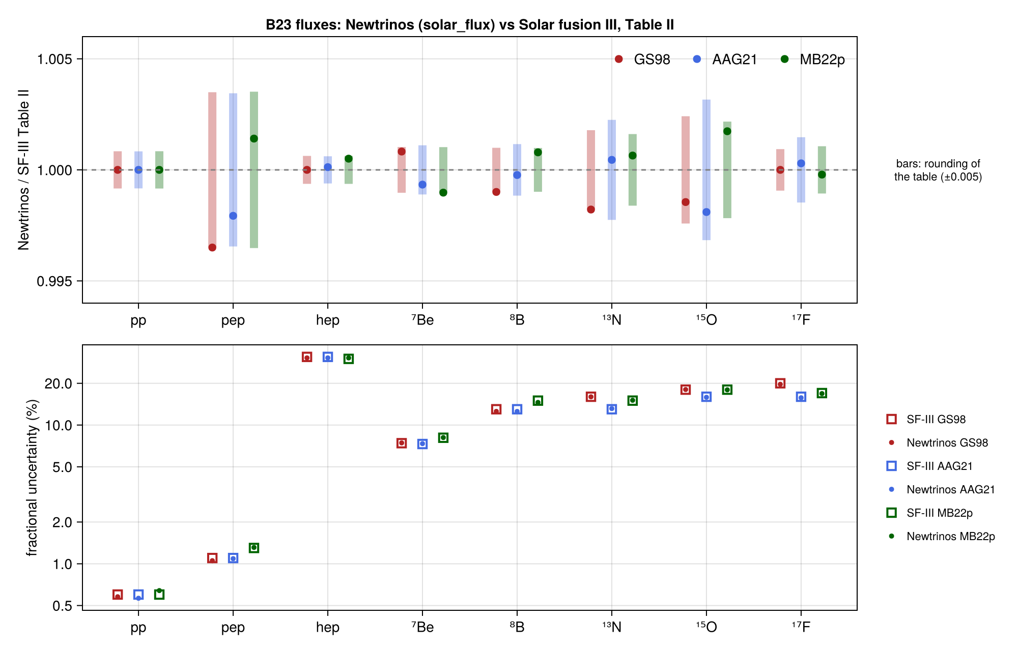
Correlation matrix of the Newtrinos flux prior (MB22m) and its difference to the B23 package · fluxes_SF3_MB22m.dat
fluxes_SF3_MB22m.dat
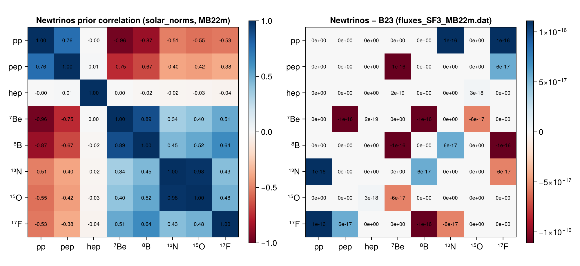
Solar electron density: B23, Newtrinos, and the previous BS05(OP) tail beyond 0.5 R☉ · struct+nu_SF3_MB22m.dat
struct+nu_SF3_MB22m.dat
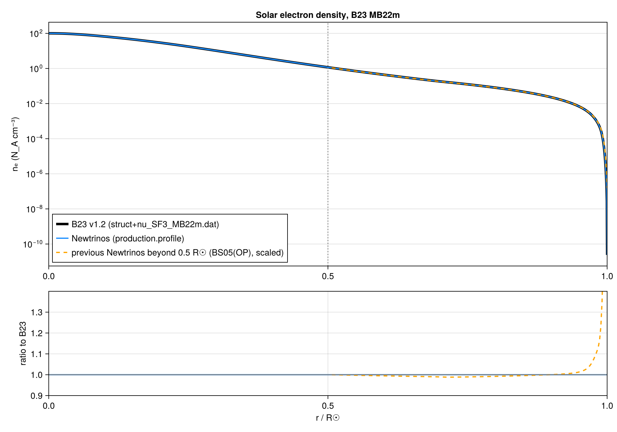
Production distributions per component: B23 vs Newtrinos' 40-point quantile compression · struct+nu_SF3_MB22m.dat
struct+nu_SF3_MB22m.dat
Known limitations
- B23 has no journal publication; the reference is the Zenodo package (concept DOI 10.5281/zenodo.10174170; Newtrinos uses v1.2, doi:10.5281/zenodo.10822316, whose structure files differ from v1.1 by up to 0.5 % in nₑ and 1–6 % in the production distributions; the fluxes are the same). The published flux values are those of Solar fusion III, Table II, which quotes B23 for GS98, AAG21 and MB22p (2–3 significant digits; the original figure is that table).
- This comparison led to a change in Newtrinos (in the pinned commit): the structure tables used to end at 0.5 R☉, and beyond it the electron density was BS05(OP) matched at 0.5 R☉. That tail was within 1 % of B23 up to 0.95 R☉ but 10 % above at 0.98 R☉, 27 % at 0.99 R☉ and a factor 2 at 0.995 R☉. Newtrinos now uses the B23 profile up to the surface. Only the non-adiabatic level crossing depends on it: the day-time P_ee changes by at most 3×10⁻⁴ (between the LOW and quasi-vacuum regions, Δm²₂₁ ≈ 10⁻⁸–3×10⁻⁹ eV²), and not at all for LMA or SMA.
- The spectral shapes (⁸B, hep, CNO, pp), the ⁷Be line branching (89.56 % / 10.44 %; Table II rounds to 90 % / 10 %) and the absorption cross sections are not part of the B23 package and are not tested here (see the BP04 and Bahcall–Krastev–Smirnov entries).
Reproduce
git clone https://github.com/Newtrinos-org/Newtrinos.jl.git && cd Newtrinos.jl && git checkout c6612c255a- Download reproduce.jl and the
data/folder of this entry into an empty directory. julia -t 8 --project=/path/to/Newtrinos.jl reproduce.jl
# Verification of the Newtrinos.jl standard solar model (module `solar_flux`, model `B23`) against the B23 / SF-III
# solar models of Herrera & Serenelli (Zenodo, v1.2, doi:10.5281/zenodo.10822316) and the B23 fluxes published in
# Solar fusion III (Acharya et al., Rev. Mod. Phys. 97, 035002 (2025), Table II).
# Run from this directory with the Newtrinos.jl environment at the pinned commit:
#   julia --project=<path to Newtrinos.jl> reproduce.jl
using Newtrinos, CairoMakie, DelimitedFiles, LinearAlgebra, Printf

cd(@__DIR__); mkpath("ours"); mkpath("results")

const SF = Newtrinos.solar_flux
const COMPS = SF.COMPONENTS
const LABEL = Dict(:pp => "pp", :pep => "pep", :hep => "hep", :be7 => "⁷Be", :b8 => "⁸B", :n13 => "¹³N", :o15 => "¹⁵O", :f17 => "¹⁷F")
const COMPOSITIONS = (:GS98, :AGSS09, :C11, :AAG21, :MB22m, :MB22p)

sf(comp) = SF.configure(SF.SolarFluxConfig(model = SF.B23(composition = comp)))
models = Dict(c => sf(c) for c in COMPOSITIONS)

# ------------------------------------------------------------------------------------------------
# B23 package flux files: fluxes, fractional uncertainties, correlation matrix
# ------------------------------------------------------------------------------------------------
function read_b23_fluxes(comp)
    lines = filter(!isempty, strip.(readlines("data/fluxes_SF3_$(comp).dat")))
    flux = parse.(Float64, split(lines[3])[1:8])
    err = parse.(Float64, split(lines[4])[1:8])
    rows = filter(l -> occursin(r"^[+-]\d", l), lines)
    corr = reduce(vcat, [permutedims(parse.(Float64, split(l)[1:8])) for l in rows])
    flux, err, corr
end

io = open("results/fluxes.csv", "w")
println(io, "composition,component,newtrinos_flux,b23_flux,newtrinos_frac_err,b23_frac_err,max_abs_corr_diff_row")
println("Newtrinos vs B23 package (fluxes_SF3_*.dat):")
for comp in COMPOSITIONS
    m = models[comp]
    flux, err, corr = read_b23_fluxes(comp)
    # correlation matrix of the Newtrinos prior on the flux normalisations (CorrelatedSSMPriors)
    Σ = Matrix(SF.ssm_prior(m).Σ)
    σ = sqrt.(diag(Σ))
    C = Σ ./ (σ * σ')
    dflux = maximum(abs.([m.nominal[c] for c in COMPS] ./ flux .- 1))
    derr = maximum(abs.(σ ./ err .- 1))
    dcorr = maximum(abs.(C .- corr))
    @printf("  %-6s max |Δφ/φ| = %.1e   max |Δσ/σ| = %.1e   max |Δρ| = %.1e   prior positive definite: %s\n",
            comp, dflux, derr, dcorr, isposdef(Σ))
    for (i, c) in enumerate(COMPS)
        @printf(io, "%s,%s,%.6e,%.6e,%.6e,%.6e,%.2e\n", comp, c, m.nominal[c], flux[i], σ[i], err[i], maximum(abs.(C[i, :] .- corr[i, :])))
    end
end
close(io)

# ------------------------------------------------------------------------------------------------
# Fig. 1: fluxes and uncertainties vs Solar fusion III, Table II
# ------------------------------------------------------------------------------------------------
t2, h2 = readdlm("data/sf3_table2.csv", ',', header = true, comments = true)
col(name) = t2[:, findfirst(==(name), vec(h2))]
unit = Float64.(col("unit"))

fig = Figure(size = (1000, 640))
ax1 = Axis(fig[1, 1], ylabel = "Newtrinos / SF-III Table II", title = "B23 fluxes: Newtrinos (solar_flux) vs Solar fusion III, Table II",
           xticks = (1:8, [LABEL[c] for c in COMPS]))
ax2 = Axis(fig[2, 1], ylabel = "fractional uncertainty (%)", xticks = (1:8, [LABEL[c] for c in COMPS]), yscale = log10,
           yticks = [0.5, 1, 2, 5, 10, 20, 50], ytickformat = v -> string.(v))
colors = Dict(:GS98 => :firebrick, :AAG21 => :royalblue, :MB22p => :darkgreen)
println("\nNewtrinos vs Solar fusion III, Table II:")
for (k, comp) in enumerate((:GS98, :AAG21, :MB22p))
    m = models[comp]
    v = Float64.(col(String(comp))) .* unit
    e = Float64.(col("$(comp)_err"))
    x = (1:8) .+ (k - 2) * 0.22
    ratio = [m.nominal[c] for c in COMPS] ./ v
    # rounding of the table: ± half a unit in the last printed digit (2 decimals)
    rnd = 0.005 .* unit ./ v
    rangebars!(ax1, x, 1 .- rnd, 1 .+ rnd, color = (colors[comp], 0.35), linewidth = 8, whiskerwidth = 0)
    scatter!(ax1, x, ratio, color = colors[comp], markersize = 11, label = String(comp))
    scatter!(ax2, x, e, color = :white, strokecolor = colors[comp], strokewidth = 2, markersize = 13, marker = :rect,
             label = "SF-III $(comp)")
    scatter!(ax2, x, 100 .* [m.fractional_error[c] for c in COMPS], color = colors[comp], markersize = 7,
             label = "Newtrinos $(comp)")
    @printf("  %-5s flux ratio %.4f – %.4f (all within rounding: %s)\n", comp, extrema(ratio)..., all(abs.(ratio .- 1) .<= rnd .+ 1e-9))
end
hlines!(ax1, [1.0], color = :gray, linestyle = :dash)
ylims!(ax1, 0.994, 1.006)
axislegend(ax1, position = :rt, orientation = :horizontal, framevisible = false)
Legend(fig[2, 2], ax2, framevisible = false, labelsize = 11)
Label(fig[1, 2], "bars: rounding of\nthe table (±0.005)", fontsize = 11, tellheight = false)
save("ours/fluxes_sf3.png", fig)

# ------------------------------------------------------------------------------------------------
# Fig. 2: correlation matrix of the Newtrinos flux prior (MB22m, the NuFIT 6.0 model) and its difference to B23
# ------------------------------------------------------------------------------------------------
m = models[:MB22m]
_, _, corr = read_b23_fluxes(:MB22m)
Σ = Matrix(SF.ssm_prior(m).Σ); σ = sqrt.(diag(Σ)); C = Σ ./ (σ * σ')
fig = Figure(size = (1000, 460))
for (j, (M, t)) in enumerate(((C, "Newtrinos prior correlation (solar_norms, MB22m)"), (C .- corr, "Newtrinos − B23 (fluxes_SF3_MB22m.dat)")))
    ax = Axis(fig[1, 2j-1], title = t, xticks = (1:8, [LABEL[c] for c in COMPS]), yticks = (1:8, [LABEL[c] for c in COMPS]),
              yreversed = true, aspect = DataAspect())
    lim = j == 1 ? 1.0 : max(1e-17, maximum(abs.(M)))
    hm = heatmap!(ax, 1:8, 1:8, M', colormap = :RdBu, colorrange = (-lim, lim))
    for i in 1:8, k in 1:8
        text!(ax, k, i, text = j == 1 ? @sprintf("%.2f", M[i, k]) : @sprintf("%.0e", M[i, k]), align = (:center, :center), fontsize = 9)
    end
    Colorbar(fig[1, 2j], hm)
end
save("ours/correlations.png", fig)

# ------------------------------------------------------------------------------------------------
# Figs. 3, 4: solar structure (MB22m): electron density and production distributions
# ------------------------------------------------------------------------------------------------
fz = "data/struct+nu_SF3_MB22m.dat"
zcols = split(strip(readline(fz), ['#', ' ', '\n']))
Z = readdlm(fz, comments = true)
zc(name) = Z[:, findfirst(==(name), zcols)]
r_b23 = zc("R_sun"); ne_b23 = 10 .^ zc("log_ne")
lerp_log(x, X, Y) = (i = clamp(searchsortedlast(X, x), 1, length(X) - 1); t = (x - X[i]) / (X[i+1] - X[i]);
                     exp(log(Y[i]) + t * (log(Y[i+1]) - log(Y[i]))))

prof = m.production.b8.profile
# the previous Newtrinos profile (up to 9112d55 … 78c8f5c): B23 up to 0.5 R☉, beyond BS05(OP) matched at 0.5 R☉
bs, _ = readdlm("data/ne_outer_bs05op_previous.csv", ',', Float64, header = true, comments = true)
scale = lerp_log(0.5, r_b23, ne_b23) / lerp_log(0.5, bs[:, 1], bs[:, 2])
r_prev = bs[bs[:, 1] .> 0.5, 1]; ne_prev = scale .* bs[bs[:, 1] .> 0.5, 2]

fig = Figure(size = (1000, 700))
ax = Axis(fig[1, 1], ylabel = "nₑ (N_A cm⁻³)", yscale = log10, title = "Solar electron density, B23 MB22m",
          yticks = LogTicks(-10:2:2))
lines!(ax, r_b23, ne_b23, color = :black, linewidth = 4, label = "B23 v1.2 (struct+nu_SF3_MB22m.dat)")
lines!(ax, prof.r, prof.ne, color = :dodgerblue, linewidth = 2, label = "Newtrinos (production.profile)")
lines!(ax, r_prev, ne_prev, color = :orange, linewidth = 2, linestyle = :dash, label = "previous Newtrinos beyond 0.5 R☉ (BS05(OP), scaled)")
vlines!(ax, [0.5], color = :gray, linestyle = :dot)
axislegend(ax, position = :lb)
ax2 = Axis(fig[2, 1], xlabel = "r / R☉", ylabel = "ratio to B23")
ok = r_b23 .<= prof.r[end]
lines!(ax2, prof.r, [p / lerp_log(x, r_b23, ne_b23) for (x, p) in zip(prof.r, prof.ne)], color = :dodgerblue, linewidth = 2)
lines!(ax2, r_prev, [p / lerp_log(x, r_b23, ne_b23) for (x, p) in zip(r_prev, ne_prev)], color = :orange, linewidth = 2, linestyle = :dash)
hlines!(ax2, [1.0], color = :gray)
ylims!(ax2, 0.9, 1.4)
linkxaxes!(ax, ax2); rowsize!(fig.layout, 2, Relative(0.3)); xlims!(ax2, 0, 1)
save("ours/electron_density.png", fig)
dev_ne = maximum(abs(p / lerp_log(x, r_b23, ne_b23) - 1) for (x, p) in zip(prof.r, prof.ne))
dev_prev = [(x, p / lerp_log(x, r_b23, ne_b23)) for (x, p) in zip(r_prev, ne_prev)]
const XS_PREV = (0.55, 0.6, 0.7, 0.8, 0.9, 0.95, 0.98, 0.99, 0.995)
@printf("\nnₑ: max |Newtrinos/B23 − 1| = %.1e over 0–1 R☉; previous BS05 tail / B23 at %s R☉: %s\n", dev_ne,
        join(XS_PREV, ", "), join([@sprintf("%.3f", lerp_log(x, r_prev, ne_prev) / lerp_log(x, r_b23, ne_b23)) for x in XS_PREV], ", "))

# production distributions: cumulative fraction, B23 tables vs Newtrinos' quantile compression (n_production points)
zname = Dict(:pp => "nu_pp", :pep => "nu_pep", :hep => "nu_hep", :be7 => "nu_7Be", :b8 => "nu_8B", :n13 => "nu_13N", :o15 => "nu_15O", :f17 => "nu_17F")
fig = Figure(size = (1000, 700))
io = open("results/production.csv", "w")
println(io, "component,b23_mean_r,newtrinos_mean_r,b23_mean_ne,newtrinos_mean_ne,b23_r50,b23_r90")
println("\nProduction regions (MB22m): mean radius and mean nₑ at production, B23 vs Newtrinos")
for (k, c) in enumerate(COMPS)
    d = max.(zc(zname[c]), 0.0)
    cdf = cumsum(vcat(0.0, diff(r_b23) .* (d[1:end-1] .+ d[2:end]) ./ 2)); cdf ./= cdf[end]
    p = m.production[c]
    local ax = Axis(fig[(k - 1) ÷ 4 + 1, (k - 1) % 4 + 1], title = LABEL[c], xlabel = k > 4 ? "r / R☉" : "", ylabel = k % 4 == 1 ? "cumulative fraction" : "")
    lines!(ax, r_b23, cdf, color = :black, linewidth = 3, label = "B23 v1.2")
    stairs!(ax, vcat(0.0, p.r), vcat(0.0, cumsum(p.w)), step = :post, color = :dodgerblue, linewidth = 2, label = "Newtrinos ($(length(p.r)) points)")
    xmax = r_b23[findfirst(>=(0.9999), cdf)]
    xlims!(ax, 0, 1.15 * xmax)
    k == 1 && axislegend(ax, position = :rb, labelsize = 10)
    trapz(y) = sum(diff(r_b23) .* (y[1:end-1] .+ y[2:end]) ./ 2)
    rm_b23 = trapz(d .* r_b23) / trapz(d); ne_m_b23 = trapz(d .* ne_b23) / trapz(d)
    rm_nt = sum(p.w .* p.r); ne_m_nt = sum(p.w .* p.ne)
    r50 = r_b23[findfirst(>=(0.5), cdf)]; r90 = r_b23[findfirst(>=(0.9), cdf)]
    @printf("  %-4s ⟨r⟩ %.4f / %.4f R☉   ⟨nₑ⟩ %.2f / %.2f N_A cm⁻³\n", c, rm_b23, rm_nt, ne_m_b23, ne_m_nt)
    @printf(io, "%s,%.5f,%.5f,%.4f,%.4f,%.4f,%.4f\n", c, rm_b23, rm_nt, ne_m_b23, ne_m_nt, r50, r90)
end
close(io)
Label(fig[0, :], "Production distributions, B23 MB22m: Newtrinos quantile compression vs the B23 tables", fontsize = 16)
save("ours/production.png", fig)
Provenance
| Newtrinos.jl commit | c6612c255a (solar_flux) |
|---|---|
| Run date | 2026-10-21T16:37:50Z |
| Wall time | 1.4 min (128 threads) |
| Julia | 1.12.5 |
| Machine | AMD EPYC 7702P 64-Core Processor, 128 hardware threads, Linux |
| Environment | newtrinos_Manifest.toml · run.toml |
Downloads
CSV files hold one row per scan point: the scanned and profiled parameters
(sin2_theta23, dm2_32 in eV², dcp in rad, nuisance parameters), dchi2 = −2Δ log L
and the log-likelihood. JLD2 files contain the full NewtrinosResult objects.
| File | Size | SHA-256 |
|---|---|---|
| ours/correlations.png | 233.0 kB | 7efd376a3b31… |
| ours/electron_density.png | 154.4 kB | a952e31ecd6a… |
| ours/fluxes_sf3.png | 150.4 kB | 8db280d774ed… |
| ours/production.png | 219.2 kB | ec64ff6a76c4… |
| results/fluxes.csv | 3.4 kB | 3d60abfb5b1f… |
| results/production.csv | 482 B | 9f37bac35a54… |